Journal · Simulation
We ran a protein folding study on a laptop to find out what the real one costs
We took a free research program we had never used before and got it running. Then we folded the same small protein 500 times. Here is what it looked like, why one run tells you nothing, and what the full 500 run job would cost on rented computers.
Our slowest run took 52 times longer than our fastest one. Same protein, same settings, same computer. The only difference was chance. That is why work like this needs hundreds of runs instead of one, why it costs money, and why a result built on a single run is worth very little. This page is the record of 500 of those runs: what they showed, what they cost, and the times our own numbers turned out to be wrong, six so far. The six points below are the short version. Everything after them is the evidence.
So: what does a protein folding simulation cost? We ran 500 coarse-grained protein folding simulations of the Fyn SH3 domain in OpenMM on one laptop, measured the throughput under a full queue, priced the same work on rented cores, and recorded what broke. This is a case study in simulation cost, numerical failure and reproducibility. It is not a result about biology.
- A protein is a tiny machine, and its shape is everything. Every living thing is full of them. Each one starts as a long chain that has to fold into the right shape to do its job, and when a chain folds wrong, people can get sick. Watching a single chain fold is near the edge of what instruments can do: it is very small and very fast, and the methods that manage it follow a few signals rather than the whole moving shape.
- So we did it in a computer instead. We took a free program that scientists wrote, and copied their experiment. We heated one protein until its shape fell apart, cooled it back down, and watched it find its shape again. The computer does this by moving every piece a tiny step at a time, millions of times over.
- We ran it 500 times, not once. Folding is partly random, so every run comes out different. Our slowest run took 52 times longer than our fastest. Running it once would have taught us almost nothing, like flipping a coin a single time and calling it.
- Here is what that bought. The 1,018-run ensemble cost about $4 to rent and 10 to 14 cents of electricity. We found that the obvious setting most people would pick runs almost three times too slow, which is the sort of thing that saves real money. And we got things wrong, six times so far, caught them, and fixed them in public instead of quietly burying them.
- What is planned would cost about $337 more to rent. Most of it is four more proteins and a ten-protein scaling run, too big for this laptop, and none of it starts until it is budgeted. A small rented run would also check that the prices on this page are real and not just arithmetic.
- And then the big one. With a real budget we would not fold one protein 500 times. We would fold thousands of proteins, or every small change you can make to a single one, and build a map of which ones get stuck and where. At ten million dollars that is 694 million runs. It is the first thing on this page that could not be done on a laptop at all, at any speed, ever. That is the whole reason renting computers matters.
If you remember nothing else: one run of anything random tells you nothing, the answer is the whole pile of runs, and that is why this kind of work is worth renting computers for.
A replica-exchange run (rex_ns188_rep2_1shf) reached: cycle 21,722 of 72,002, 30.2 per cent, 15 temperature windows from 293 to 450 K, moving at 3,288 exchanges an hour. About 15.4 hours left. Exchange acceptance is running between 0.17 and 0.79.
The machine is giving it 11.0 of 18 cores, load average 16.9, and the graphics card is idle. Idle on purpose: the batched GPU path is validated but this run is replica exchange, and the engine that would put replica exchange on the GPU failed its physics check. More on that below.
Measured at 2026-10-30 21:38:05 UTC and frozen there. This page does not update itself, so
reload it to see whether these numbers have moved.
livestatus.py writes these figures on every run.
What is running right now
21 finished, 1 in flight, 1 stopped, 0 failed, 4 ready to start and 4 queued behind them. This is the whole programme, not just tonight: every planned run is here, including the ones that may never happen. A full bar is work that completed, including the runs we later withdrew; an empty one has not started. The bars are read from each run's own files every fifteen minutes, not typed by hand, so they are as current as the timestamp underneath. A bar that stops moving means a run stopped, and that is worth knowing too. Queued rows show when they can start, or what is blocking them; two of them are waiting on binaries we do not have and may never start at all.
The first full run. Superseded by v2 on a 13-window ladder reaching 293 K.
The run every published 1SHF number comes from. 34 round trips, minimum pair acceptance 0.595. Its stability was tested against Plaxco 1998 and missed by 3.4 standard deviations.
Found the ladder severed at the folding transition: pair 9-10 acceptance 0.080, zero round trips in 2,002 exchanges. The ladder was mis-designed.
The direct test of tonight's reweighting result. Reweighting predicts the Go model reaches the published -6.0 +/- 0.6 kcal/mol at nscal about 2.0, against -3.91 at the 1.4962 in use. This run measures it with no reweighting assumption, on a force field already fitted and on disk. 17 windows, 293 to 470 K, bracketing a melting point measured at 430.5 K.
Queued automatically behind the 2.0322 run. Two measured points either side of the value in use test whether the reweighting predicts dG across the range, which is the 7.3x saving that would make the card set locally feasible. Ladder bracketing a melting point INTERPOLATED between two measured ones, not extrapolated: extrapolation was 48 K wrong for 2.0322.
The rerun that can deliver the stability comparison. The first 3CLA run already gave a melting point of 345.45 K against a published 341.2 K; what it could not give was the stability at 298 K, because its ladder bottomed at 306 K. This one reaches 296 K so the published temperature is bracketed, and keeps the five transition windows that resolved 2% to 98% unfolded.
Extends the dG-versus-nscal curve well below the three measured points, which is the real test of whether it is linear. At this force-field strength the melting point drops to about 307 K, so the ladder runs from 270 K to hold a folded population at the experimental temperature at all.
The capstone of the force-field thread. Four measured runs give a curve whose quadratic fit, as it stood on 23 October, said nscal 1.882 should reproduce Plaxco's -6.0 (the curve corrected on 25 October says 1.890) kcal/mol. This force field was BUILT for that prediction, with the patched model builder, and had never existed before. If it lands near -6.0 the calibration predicts rather than merely describes. FINAL at 216,014 exchanges, six times the first run: -6.039 +/- 0.069 kcal/mol against a published -6.0 +/- 0.6, so z = -0.06. At 36,002 it was -5.979 +/- 0.115. The effective unfolded count at the published threshold rose from 1.06 to 5.76, against about 6.4 predicted for proportional growth, so the cold window was thin, not trapped, and the ladder made 414 round trips against 70. The agreement holds with six times the sampling. What this test could show is limited, and should be said: the calibration runs either side of 1.882 (1.7453 at -5.303, 2.0322 at -6.597) already agree with -6.0 within Plaxco's +/- 0.6 on their own, so any result between them would have agreed. It confirms the curve; it could not have refuted the model. An independent repeat with a different seed is now running, against a pass criterion published before it finishes.
PDB 2CI2 chain I, residues 20-83, 64 beads, 60 native contacts. 2CI2 was chosen over 1COA and 1YPA because those are engineered mutants; 2CI2's own unresolved residues are an N-terminal tail outside the folded domain, so the deposited structure and the construct the folding literature uses agree. That construct check is what killed the 1998 Fyn SH3 recreation. It runs at nscal 1.882, the value calibrated on 1SHF, making this a test of whether the calibration TRANSFERS between proteins. RESULT: it does not. At nscal 1.882 CI2 reaches -2.760 kcal/mol against a published -7.03 ± 0.16, z = 26.5. The folded-state threshold was swept across 6 values because there is no published one for CI2, and the disagreement runs from z = 16.0 to z = 36.5, so the conclusion does not depend on that choice. The run made 167 round trips, so this is the force field, not short sampling.
306 beads, the largest protein with a fitted force field on disk, and the only carded protein with no result. Ladder placed from a measured melting point rather than guessed: the scan put the Q = 0.5 crossing at 373.3 K, bracketed between 370 K at Q = 0.564 and 385 K at Q = 0.269, and the 16 windows run geometrically from 293.15 K, the experimental target temperature, to 418.27 K. 4C5C runs at nscal 1.0, below every other carded protein, so neither 3CLA's toolkit ladder nor CI2's 371 K would have transferred. A first ladder was stopped at cycle 629 of 36,004 and is kept: its measured pair acceptance collapsed to 0.076 and 0.049 on the two pairs straddling the melting point, against a median of 0.572. That acceptance profile alone was the reason: 0.049 in series with 0.076 makes traversal of the ladder very unlikely. It had also made zero round trips, but at 608 cycles that is NOT diagnostic, because a round trip across 16 windows needs of order 1,250 cycles even at healthy acceptance, so zero was expected either way and is not cited as evidence. The ladder was redistributed from the measured acceptances rather than guessed again: windows clustered through the transition, the cold end stretched, still 16 windows and 16 cores. That moved the worst pair from 0.049 to 0.193 over 36,004 exchanges, with 1 pair now below the 0.20 band. An earlier reading of 0.134 was taken at 642 cycles, about ten attempts per pair, and was small-sample noise. Round trips 0 at 36,004 exchanges. Spans 9 to 16 of 16 windows, and 1 of 16 replicas have reached both ends. The limiting boundary is now 5 to 6, accepting 0.193 and carrying only 43.0% of the median crossing traffic. 🔴 A free random walk at the observed move rate would complete a round trip in about 926 exchanges, and this run is 39 times past that with none completed. One replica crossing once is not mixing. UNKNOWN whether longer sampling closes this; the board's standing item on a sampling method that can cross a first-order transition is the alternative. Free energies pooled from these windows must NOT be read as converged.
One stage is still blocked on a binary we do not have: pd2_ca2main, which gates verifying backmapping against its shipped reference. The Linux-only ribosome_traffic that blocks continuous synthesis has a route: a linux/amd64 container is built, but that example has not been rerun in it yet. Every one of the 20 has been attempted: 2 run but have no usable reference, 2 do not run here, 1 runs and does not reproduce.
The stopped run ALREADY gives a melting point: 345.45 K against the published 341.2 K, a difference of +4.25 K. Round trips were the wrong convergence test; the per-window populations are stationary, which is what actually matters. What is missing is the stability at 298 K, because that ladder bottomed at 306 K. This one reaches 296 K so the published temperature is bracketed, and keeps the five transition windows that resolved 2% to 98% unfolded. The stability target is the only EXACT external number we hold: -8.4315 kcal/mol at 298 K, published by the toolkit's authors before we started.
Our 1SHF stability missed Plaxco 1998 by 3.4 sigma. opt_nscal optimises a binary 'is it stable' criterion that does not pin a free energy, so this asks whether the model class can reach -6.0 at all, and at what nscal. RESULT: by reweighting, the Go model reaches the published -6.0 +/- 0.6 kcal/mol at nscal about 2.0, against -3.91 at the 1.4962 in use. Reweighting was later found to understate stability by about 0.6 kcal/mol at nscal 2.03 (stability_ns2.0322.json), and the direct runs put the crossing near 1.89. Either way the 3.4-sigma miss is not a limit of the model class; opt_nscal's binary 'is it stable' criterion is satisfied anywhere above about 1.3, across which the free energy still varies by 3.4 kcal/mol.
CLOSED, and not by building anything. PDB 1NYF and 1NYG ARE the 67-residue construct, human Fyn, solution NMR, no mutations. They span residues 82 to 148 but resolve only 84 to 141: the eight extra residues are disordered tails at both termini. A coarse-grained model is built from the native contact map, and disordered residues contribute none, so a 67-mer model would be essentially identical to the 59-mer we already have. This REFUTES the construct explanation for the 3.4-sigma stability miss and leaves the force-field strength, which independently reproduces the measurement at nscal about 1.9.
The heat capacity computed from energy FLUCTUATIONS must equal the one computed from dE/dT. That is exact for any canonical ensemble: no model, no fit, no literature value to be wrong about. It tests whether replica exchange is sampling Boltzmann at all, which every comparison to experiment silently assumes. Result: 9 of 11 interior windows agree within 25 per cent, median ratio 0.918 against an exact 1.000. The two that disagree both sit beside a 20 K gap in the ladder, where the numerical derivative is least accurate, so the shortfall tracks the finite difference rather than the sampling.
Turns the force-field strength from a fitted guess into a measured quantity. The fourth point showed the relation is mildly CURVED, not linear: a line leaves residuals of +0.18, -0.19, -0.18, +0.19, a systematic U shape. Three points could not have revealed that.
Unblocks stage 3: ribosome_traffic is a Linux x86-64 binary with no source and cannot run on this machine. Built period-correct (OpenMM 7, older numpy) it would also run the toolkit on the versions it was written for, separating 'the toolkit is broken' from 'it has not been run on current software in years'. Does NOT fix pd2_ca2main.
Planned 2026-10-24. The journal page is 32,000 words and becomes the full RECORD; a summary page becomes the landing page. One piece is being drafted early rather than late: 'what we learned' rests on the sequence of corrections, and the result files record the final answer without recording that we were wrong first. The headline is gated on CI2: if it lands where the calibration predicts, the summary is about a transferable method; if not, it is about one protein. Those are different articles.
Eight temperatures from 300 to 400 K, 1,200,000 steps each, matching the step count of the CI2 scan on record. One process per temperature, which is bit-identical to tscan.py's serial loop because it seeds each temperature as seed plus the temperature. This gates the queued 4C5C production run: replica exchange only samples if its windows bracket the melting point, and 4C5C runs at nscal 1.0, below every other carded protein, so neither 3CLA's toolkit ladder nor CI2's 371 K transfers. A scan and not a measurement: near the melting point the chain flips slowly, so a short run understates unfolding and the crossing is approximate. COMPLETE: melting temperature approximately 373.3 K, ladder can now be placed.
Every 1SHF free energy published here was computed at Q >= 0.75 and nowhere else, and the headline result rests on it. Swept across eight thresholds on all five existing trajectories. RESULT: the calibrated force-field strength ranges 1.4833 to 2.2002 from the threshold alone, against 1.882 as built, and the prediction agrees within two sigma at 3 of 8 thresholds. At the published threshold the first 36,002 exchanges rested on about one effective unfolded configuration; the run was extended to 216,014 and that rose to 5.76, with the answer unchanged (see the 1.882 row). The threshold dependence itself is not removed by more sampling and still applies to every 1SHF number here.
Every uncertainty published here resamples blocks of frames while reusing one set of MBAR free energies solved once on the full data, which treats a fitted object as if it were known. This re-solves MBAR inside every resample and reports the ratio to the cheap estimator, at the published threshold and at a well sampled one.
The prediction test landed within 0.04 kcal/mol of Plaxco's -6.0 with 216,014 exchanges. One run can agree by luck, so this one starts it again from scratch with a different random seed. It is compared with the first run, never pooled with it. If the two agree, the result does not depend on which random path the simulation happened to take. If they disagree, that is the finding. PASS CRITERION, registered 2026-10-30 21:36 UTC at cycle 21,600 of 72,002, before any analysis of this run: compare with -6.039 kcal/mol at Q >= 0.75 by the same analysis. Each run's uncertainty is the larger of its bootstrap error and a counting floor of RT over the square root of its effective unfolded count, so the reference counts as +/- 0.243, not +/- 0.069. PASS if the two differ by under 2 combined sigma; FAIL at 2 or more, reported as the finding. INCONCLUSIVE, with no agreement claimed, if this run's effective unfolded count is below 1; about 1.9 is expected. This tests reproducibility across seeds, not the calibration.
Stopped deliberately 2026-10-21 at ~24,100 of 60,002 exchanges, 18.5 h in. Reason: ZERO round trips. Pairwise acceptance was healthy throughout (min 0.56, median 0.71) but acceptance is not mixing: a replica can swap temperature every cycle and still never cross the folding transition, which requires the chain to physically unfold and refold. The 7 half-traversals all occurred in the opening phase while replicas were still leaving the native start; mixing then stopped. Reaching ~10 round trips per replica would need >3.6 million exchanges (~2,775 h). The run is resumable from state.json if tha
Runs inside the linux/amd64 container, because ribosome_traffic is a Linux x86-64 binary. The earlier stage 3 attempt on this machine ran with that path switched off, so it is not comparable to the reference.
Model building was unblocked tonight by the OpenMM 8 fix. The expensive step is fitting its own nscal: one full replica-exchange run per candidate value.
The only route to verifying stage 5. The shipped backmapping reference was built PD2-then-pulchra and we have no copy of PD2 for any platform. Until it arrives, 6 of 6 is unreachable and 5 of 6 is the ceiling.
The gate on 3CLA and 4C5C, and therefore on proteins above about 200 beads. Plain temperature replica exchange made zero round trips in 24,096 exchanges with healthy acceptance, because the barrier is latent heat rather than ladder resolution. Candidates are multicanonical, Wang-Landau or well-tempered metadynamics. None is implemented here.
Matched to the authors' own 3,180,000-step reference run.
Running without ribosome traffic: that binary is Linux x86-64 only, so this path differs from the reference.
The shipped reference was built PD2-then-pulchra. Until that binary is sourced this stage can be run but never compared.
All six modules in sequence on verified code. Run on 1SHF because it is the only protein where we hold an independent external number to check the end of the chain against.
Ten proteins use 150 cores genuinely concurrently. Deliberately NOT a single large protein: that is 25,637 core-hours against a ~15-core ceiling, 71 days, with 985 of 1,000 rented cores idle.
33.6 days on this machine against 4.8 days rented. The cost is about $252 at spot; the constraint is wall clock, not money.
core-hours, summed across every finished, running and queued run. Core-hours add up; wall hours do not, because runs overlap, so the completion time below is the longest remaining run rather than a sum. Counted across 15 finished, running and queued runs. 18 further items on this list are analysis rather than simulation and carry no core-hour cost.
Read at 2026-10-30 21:38 UTC. timeline.py; each bar is read from the run's own files.
The set: one card per protein
Three proteins ship with a fitted force field in the toolkit we are using. We have folded two of them. We also built a fourth protein ourselves, CI2, which the toolkit does not ship, specifically to test whether what we learned on the first one transfers. All four are here. The bars are measured for every card, because size and raw throughput were benchmarked before anything was folded; the results fill in as each run lands.
The sizes matter more than the names. 59, 64, 213 and 306 beads is a five-fold range, and size drives everything else on this page: cost per step, where the graphics card stops helping, how many copies fit in one context before throughput collapses, how long a fold takes, and whether replica exchange can cross the folding transition at all. That last one cost us a run.
Every number on a card carries a tag saying where it came from. Two of the five tags are the ones that matter for whether any of this is believable:
The labels carry the verdict, not just the fact that a comparison happened. On the SH3 card the model is tagged Not replicated at the force-field strength the toolkit ships, and Provisional at a strength 36 per cent higher, where it agrees but rests on under one effective unfolded configuration. Both are on the card, because the gap between them is the finding. Each card has a line you can open giving the full accounting.
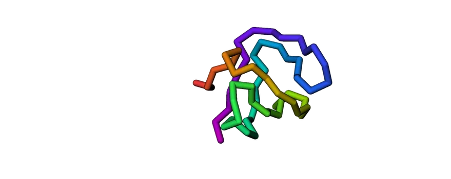
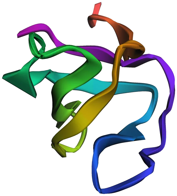
The grip of a human signalling enzyme. Small, fast, reversible, and measured in laboratories since the 1990s.
Agrees at the calibrated strength, NOT replicated at the 1.4962 the toolkit ships
The model MISSES the published stability at the force-field strength the toolkit ships, and REPRODUCES it at a strength 36% higher. Both runs are on this card because the gap between them is the finding.
- Not replicated Folding free energy at 293.0 K is -3.91 ± 0.10 kcal/mol. The laboratory value at 293.15 K is -6.0 ± 0.6. The model is 2.09 kcal/mol less stable than the real protein, a disagreement of 3.4 standard deviations. The replica ladder was verified mixed first (34 round trips), and the 40 unfolded frames the estimate rests on fall in 37 independent episodes.stability.json · doi:10.1021/bi972075u
- Provisional The same model at nscal 2.0322 gives -6.60 ± 0.16 kcal/mol against the laboratory −6.0 ± 0.6, z = -0.96. Pooled across all 17 windows by MBAR. Two caveats, both ours: this point did not discard the first quarter as equilibration, unlike the other three calibration points, and done that way it is -7.033 ± 0.153 kcal/mol; and at 293 K it rests on 0.19 effective unfolded configurations, under one, so it is provisional. So the model class was never the problem: the toolkit fits nscal to a binary 'is it stable' test that is satisfied anywhere above about 1.3, across which the free energy still moves 3.4 kcal/mol.stability_ns2.0322.json · 36,002 exchanges, 99 round trips
- Ratio, not a test The 0.91 million-fold speed figure is a ratio of our folding time to the published one. It says how much faster simulation is than a laboratory, not whether this model folds correctly.
- Never tested Both melting points, all folding times and the folded fraction remain this model's own output. No published melting point for 1SHF has been located to test them against.
- Ruled out The construct difference was the obvious suspect and is not the answer. PDB 1NYF is the 67-residue construct Plaxco measured: it spans residues 82 to 148, but only 84 to 141 are resolved. The eight extra residues are disordered tails that form no native contacts, so a coarse-grained model of the 67-mer would be essentially identical to this one. That leaves the force-field strength as the explanation, which reproduces the measurement at nscal about 1.9.PDB 1NYF and 1NYG, solution NMR, zero mutations
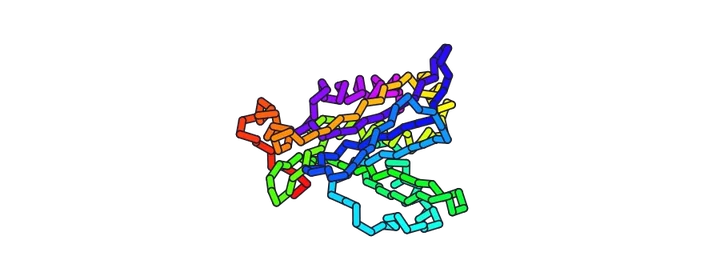
An antibiotic-resistance enzyme. Its melting point sits 2.83 K from the toolkit's own value, and its stability agrees provisionally, on thin sampling from a run that never mixed.
Matches the toolkit's own simulation, provisionally
The toolkit's authors published two numbers for this protein, computed with their own simulation rather than measured in a laboratory. Matching them tests whether we run their model the way they did, not whether the model matches nature.
- No verdict possible Melting point 344.03 K against the published 341.2 K, a difference of +2.83 K. Measured on a 16-window ladder reaching 296 K, improving on +4.25 K from a coarser ladder. The run made ZERO round trips, but the per-window populations are stationary across the second half, and that is the criterion that matters: round trips are sufficient for convergence, not necessary. The published 341.2 K carries no stated uncertainty, so agreement cannot be tested statistically: +2.83 K is a difference, not a demonstrated disagreement.stability_3cla_v2.json · 24,002 exchanges
- Provisional Folding stability -7.42 ± 0.86 kcal/mol against the published -8.4315, a difference of +1.02 at z = +1.18. Measured with the toolkit's own criterion, Q ≥ 0.7321, pooled across all 16 windows. Provisional, not replicated: at 298 K it rests on 0.04 effective unfolded configurations, and the run made zero round trips, the same condition under which the 4C5C card declines to quote any free energy at all.stability_3cla_Q.json
- Withdrawn An earlier attempt returned −20.8 kcal/mol from the same trajectory and the same windows. Only the folded-state criterion differed: an energy proxy instead of Q. That one choice moved the answer by 13 kcal/mol, which is the whole lesson.superseded 2026-10-24
- Recovered The coordinate file this needed had been deleted by a temporary-directory sweep. It was restored from a surviving git pack, along with 458 other toolkit files.

The reference two-state folder, and the only card chosen to test the method rather than the protein. It runs at the force-field strength calibrated on the SH3 domain, so it asks whether that calibration transfers between molecules at all.
The calibration does not transfer
This card asked whether the strength calibrated on the SH3 domain carries to a molecule it has never seen. It does not. At nscal 1.882 CI2 reaches -2.760 kcal/mol against a published -7.03 ± 0.16. It agrees with the published value at 0 of the 6 folded-state thresholds tested.
- Result Q ≥ 0.65 gives -4.399, z = 16.0; Q ≥ 0.7 gives -3.596, z = 21.1; Q ≥ 0.7321 gives -3.018, z = 24.8; Q ≥ 0.75 gives -2.760, z = 26.5; Q ≥ 0.8 gives -1.959, z = 31.6; Q ≥ 0.85 gives -1.181, z = 36.5. The model gives CI2 roughly 39 per cent of its measured stability at the threshold used everywhere else on this page.stability_ci2.json
- Why six thresholds and not one Choosing which configurations count as folded is the most consequential free choice in this project, and one such choice once moved an answer by 13 kcal/mol. There is no published threshold for CI2, so rather than pick one and present it as the answer the whole plausible range was swept. The disagreement runs from z = 16.0 to z = 36.5, so the conclusion does not depend on the choice. That is the only reason it is stated.stability_ci2.json
- The error bars are not what carries this The quoted uncertainties are block-bootstrap statistical errors at a fixed threshold, and they EXCLUDE the threshold systematic, which this sweep measures at about 16 kcal/mol per unit Q and which is therefore far larger. The refutation does not rest on them: the gap is 4.27 kcal/mol, so it survives inflating every error bar by an order of magnitude. A z of 26 is not a claim that the uncertainty is 0.021.stability_mbar.py
- Not a sampling failure The run made 36,002 exchanges and 167 round trips, a per-replica median of 10, which is the test an earlier run in this project failed with zero. The ladder mixed. This is the force field being wrong for this molecule, not the sampling being short.mixing.json
- What it does not establish That calibrations never transfer. One transfer was tested, between two small two-state folders, and it failed decisively. It also does not establish WHY: whether the force field, the contact map, the absence of solvent or something particular to CI2. The pH and temperature caveats below are real and are ours, and neither explains a gap this size.
- Target verified Jackson and Fersht 1991 give a folding free energy of 7.03 ± 0.16 kcal/mol by guanidinium denaturation and 7.18 ± 0.43 by thermal denaturation, at pH 6.3. Read from the primary abstract rather than taken second hand.doi:10.1021/bi00107a010 · PMID 1931967
- Caveat on the target That figure is quoted at pH 6.3 and extrapolated to zero denaturant. Our model has no pH, no titratable groups and no solvent. The abstract also does not state a temperature; 298.15 K is assumed and that assumption is unverified.ci2_published.json
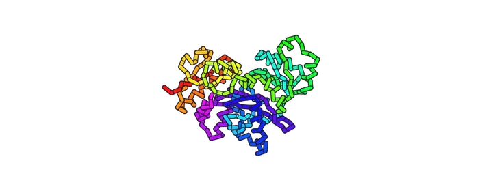
The largest protein with a fitted force field on disk, and the most expensive per step of the four.
No published value to compare against
No independent measurement of this protein's folding has been located, so nothing here can be compared. Every figure on this card is a property of the structure, a projection of cost, or a statement about how the run sampled.
- Derived Bead count and contact cost come from the deposited structure and from throughput measured on this machine.
- Projected The arrival estimate scales a measured rate. It is a forecast, not a result.
Read as of 2026-10-30 21:38 UTC. The countdowns tick in your browser from a target timestamp baked into the page; the hours are an estimate from measured throughput, not a promise.
The code
The toolkit is cg_simtk_protein_folding from the O’Brien Lab at Penn State, written by Yang Jiang. It is a coarse-grained simulation package for protein folding, and it is the software behind five published papers, including work in Nature Communications, Nature Chemistry and Science Advances.
Counted in the clone: 36 Python scripts, 15 Perl scripts and 2 Tcl rendering scripts, 23,556 lines between the Python and the Perl. It is a research codebase rather than a product, which is the normal condition of scientific software and the reason this kind of work needs setting up at all.
The physics it runs is a Cα Gō-like model. Each amino acid becomes a single bead at the position of its alpha carbon, and the pairs of residues that touch in the known folded structure are given attractive interactions while everything else is repulsive. It is a deliberate simplification. It buys a timestep of 15 femtoseconds against the 2 femtoseconds a typical all-atom simulation uses, and it drops the solvent entirely, which together are what make folding reachable at all on this budget.
We still have not run their pipeline end to end on one system. Five of the six protocol directories are runnable on this machine and the sixth is reachable with a substitute, but runnable is not the same as run: the continuous-synthesis and post-translational folding directories have had no example put through them at all, and 13 of the 20 shipped examples are still unattempted.
Three of the tools the workflow expects are absent and substituted rather than satisfied: Stride by a pydssp shim, PyEMMA and msmtools by a compatibility layer onto deeptime, WHAM by pymbar. Substitution is not emulation, and this article says where each one differs. CHARMM, MATLAB and VMD are absent with no substitute; none of them blocks a stage.
One comparison we cannot make at all. The backmapping example runs here after patching, but its shipped reference was produced with pd2_ca2main, which is not installed and which we have no copy of for any platform. That example runs and cannot be checked, which is a different thing from passing.
Why this protein
The molecule in every picture on this page is a small piece of a human protein called Fyn. Fyn is an enzyme that passes signals around inside cells, and the piece we are folding is one of its parts: an SH3 domain, 59 amino acids long. Its structure was solved by X ray crystallography in 1993 and sits in the public database as entry 1SHF, measured to 1.9 Å.
SH3 domains do a simple job in the cell. They are the part of a larger protein that grips onto other proteins, so the right things meet at the right time. Our simulation says nothing about that job. We are not studying what this domain does. We are studying how it finds its shape.
It is the fruit fly of protein folding
Small domains like this one are the standard test subject for folding research, and the reason is worth understanding, because it explains the whole shape of this piece.
A protein that folds in seconds is hard to simulate and hard to measure. One that falls apart and reassembles quickly, reversibly, and the same way every time can be watched in a laboratory and reproduced in a model. SH3 domains do that. They are small, they fold fast, they come apart cleanly when heated, and decades of experiments have measured how stable they are and how quickly they fold. That makes them one of the few systems where a model’s answer can be checked against a real one.
So this protein is not the question. It is the ruler. You calibrate a method on something whose answer is already known, find out where the method goes wrong, and only then point it at something nobody has measured. The toolkit ships it as the worked example for its quenching protocol, and a run like ours is worth doing even though it discovers nothing new about Fyn.
What work like this is for
Proteins that fold wrongly are behind a long list of diseases, and a protein that gets stuck on the way to its shape is a different problem from one that never had the right shape available. Telling those apart needs models that can be trusted, and models earn trust by being tested on molecules like this one. None of that is a claim about Fyn, which is not a protein this work says anything about.
What we actually did, in plain words
If the rest of this page is heavy going, this is the whole thing in one section. No equations and nothing you need to look up.
The thing we are copying
A protein is a long chain. A cell builds it in a line, like beads threaded on a string, and the moment it exists it collapses into a specific knot. That knot is the protein. The chain is useless; the knot does the job. Our chain is 59 beads long and its knot is a small clamp that holds other proteins.
Nobody fully understands how a chain finds its knot. There are more ways to fold a chain than there are atoms in the universe, and a real protein does it in about a millionth of a second. Watching it happen in a laboratory is close to impossible: it is far too small and far too fast.
So we do it in a computer instead
We write down where every bead is, work out how hard every bead is pulled by every other bead, move them all a tiny step, and do it again. The step is fifteen femtoseconds, which is fifteen millionths of a billionth of a second. To cover the first hundred nanoseconds of a protein’s life takes about seven million of those steps.
That is all a molecular simulation is. An enormous number of very small, very boring steps.
The experiment: break it, then watch it mend
You cannot watch a chain fold unless it is unfolded first. So the experiment has two halves.
Heat it up. We set the temperature to 1000 K, which is hotter than molten lead. The knot shakes itself apart within a fraction of a nanosecond and the chain flails as a loose string. This is not something that happens in a cell. It is a way of getting a clean starting point, like unknotting a shoelace before timing somebody tying it.
Cool it down. We drop the temperature to 310 K, which is body heat, and then we do nothing except watch. Left alone, the chain finds its knot again. We record how long that takes.
That is one run. One number: how many nanoseconds to fold.
You have felt this happen, in a small way
The 310 K we cool to above is 37 °C, ordinary body heat. When you catch a cold, your body turns its own thermostat up. A fever takes you to 38 or 39 °C, a rise of a degree or two. That is nowhere near the 1000 K we use to pull a protein apart, and it is worth being clear that a fever does not work by melting the virus. What it does is quieter, and it is the same balance this page measures.
A folded protein is only just more stable than an unfolded one. The margin is a few kilocalories per mole, which is a very small amount of energy: it is the number we spent most of this project measuring, and for the protein on this page it is about 6. With a margin that thin, a degree or two genuinely shifts the odds, and the proteins in your own body spend a little more of their time loosened. Your cells notice and respond by making heat shock proteins, which work as minders: they catch proteins that are starting to come undone and help them back into shape.
The fever fights the infection in other ways. It speeds up parts of your immune response, and the most common cold viruses multiply best at the cooler temperature inside your nose, so warmth puts them at a disadvantage. The fever is not breaking the invader apart. It is tilting a very fine balance in your favour, and how much heat it takes to tip a folded protein into an unfolded one is exactly what the experiments on this page measure.
Why do it 500 times?
Because the answer is different every time. Not slightly different. Our slowest run took 52 times longer than our fastest, with nothing separating them but the random kicks the thermostat applies. There is no water in this model: the solvent is a random force and a drag, which is where the randomness comes from. One run tells you almost nothing, the way one coin flip tells you nothing about a coin.
So the result is never a single trajectory. It is the shape of the whole pile of them, and that is why a question like this costs money: you are not buying one answer, you are buying enough answers to know what the answer looks like.
And why would anyone want this?
Because proteins that fold wrongly cause disease, because drugs are made of proteins that have to fold correctly in a factory, and because the only way to know whether a computer model of folding can be trusted is to run it on something whose answer we already know and check. That is what this page is: a careful check on a model, run by people who had never used it before, with every number and every mistake written down.
Standing it up
The repository targets OpenMM 7.4.1 with CUDA 9.0 and Python 3.7, tested on RHEL7 and CentOS7, on a cluster. We ran it on a laptop. The force field, topology and native coordinates loaded unchanged, and the native structure scored Q = 1.00 against the toolkit’s own contact definition, which is the check that we were reading the same geometry the authors were.
| Measured on | |
|---|---|
| Machine | Apple M5 Max, 18 cores, 6 performance and 12 efficiency |
| Graphics | 40 core integrated GPU, no CUDA device |
| Memory | 128 GB unified memory |
| Operating system | macOS 26.4 |
| Software | Python 3.14, OpenMM 8.6.1, numpy 2.5.4, ParmEd 4.3.1 |
| Steady-state rate | 3,750 steps/s per core, 18 processes at once |
| Date | 18 October 2026 |
That table is there so every number below has a stated baseline, not because the machine is interesting. It is a well specified laptop and it is still a laptop: no part of the method needs it. The same code runs on a cheaper machine more slowly and on rented cores faster, and the whole argument of this piece is that the second of those is usually the one worth buying. Where a figure depends on the hardware we say so, because a core here is not a core somewhere else.
One genuine break. minimizeEnergy took an energy tolerance in
OpenMM 7 and takes a force tolerance in OpenMM 8, so the original call raises a
TypeError about incompatible units. One line, and the kind of thing
a six year old research code will always have.
The second finding cost an afternoon and is the one worth the money.
Picking the backend is worth more than it sounds
OpenMM can run on several compute backends. The obvious choice on a machine with no GPU is the multithreaded CPU platform. For this job it is less than half as fast as the plain single-threaded Reference platform that exists mainly as a correctness check, and the reason it loses is instructive.
| System | Beads | Reference | CPU platform | Winner |
|---|---|---|---|---|
| SH3 domain1SHF, 18 at once | 59 | 77,848 | 30,448 | Reference, 2.6× |
| Acetyltransferase3CLA, 18 at once | 213 | 16,743 | 13,652 | Reference, 1.2× |
| DDLB ligase4C5C, 18 at once | 306 | 10,262 | 7,814 | Reference, 1.3× |
| Truncated 50S and tRNAone job, all 18 threads | 4,577 | 43 | 388 | CPU, 9× |
Aggregate steps per second, measured on 18 October 2026. The advantage inverts. Running many small systems at once, a force evaluation is cheaper than the thread pool’s own synchronisation, so eighteen pools spend their time waking each other up and the backend with no pool wins by 2.6 to 1. Running one large system, the pool finally has enough work to divide and the same backend loses by nine to one. Run a single trajectory alone on an idle machine and the two land within two per cent of each other, which is exactly why the benchmark most people run shows none of this.
The other half of the machine was simply not being used. OpenMM will talk to the integrated GPU through OpenCL. Adding eight GPU contexts alongside the CPU processes took the whole machine to 77,117 steps per second. Against the matched baseline, the same 18 CPU processes without the GPU at 67,504, that is a 14 per cent gain for work the GPU was idle through anyway. We first reported 18 per cent by comparing against a 16 process run, which credits the graphics card with two processor cores it did not provide; the honest comparison changes one thing at a time. A GPU worker costs about a fifth of a CPU core to host, so it is close to free capacity.
One more trap, found the hard way while this ensemble was running. Constructing an
OpenMM Simulation spawns a thread pool sized to the machine, eighteen
threads here, whatever platform you asked for, and no combination of
OPENMM_CPU_THREADS, OMP_NUM_THREADS or the rest turns it off.
Our driver builds two per trajectory, one to unfold and one to refold. Twenty six
trajectories at once therefore meant about nine hundred and sixty threads competing for
eighteen cores, a load average of 162, and a laptop too busy to render a web page. Cutting
to eighteen workers made the whole ensemble finish sooner. More workers are not more
throughput once the threads outnumber the cores by fifty to one.
None of these factors is visible in the benchmark most people run, which is one process on a quiet machine. Measure the throughput of the whole ensemble under the load the real job runs at, on the system size you actually have. Between the backend choice and the idle GPU there is a factor of two and a half on this job, and that is a factor of two and a half on the bill.
Mixing backends inside one ensemble is only legitimate if they agree on the physics, so we checked rather than assumed. On the native structure the three backends return a potential energy of −56.3096, −56.3096 and −56.3095 kcal/mol, agreeing to within 1.6×10⁻⁵, and all three score Q = 1.00 after minimisation. The trajectories below were produced on both CPU and GPU, and each one records which.
When a graphics card is the right machine, and when it is not
The obvious accelerator loses twice on this page, and an anecdote that happens twice is worth turning into a rule. A timestep is a hard sequential barrier: step n + 1 needs the positions from step n, so no hardware parallelises across time. That leaves exactly two places to find concurrency, and the two machines are built for different ones. A processor is eighteen independent cores, each quick on its own, which suits eighteen unrelated jobs. A graphics card is one very wide pipeline, thousands of lanes behind a single dispatch, which suits one job with thousands of simultaneous bodies and is wasted on 59. The question is never which chip is faster. It is which kind of concurrency the experiment has.
The arithmetic is blunt. At 59 beads and 50 native contacts a single step is on the order of a hundred thousand floating point operations, which a forty-core GPU could finish in nanoseconds. The measured cost of a step on that GPU is about fifty microseconds. So arithmetic accounts for a vanishing fraction of the step and something other than arithmetic accounts for essentially all of it, and a wider card would not change a digit of that.
Be careful how far that goes, because we have bounded the arithmetic rather than measured the rest. Kernel dispatch, host-to-device transfer, thermostat and constraint kernels, and synchronisation are the usual suspects, and this page has not profiled them separately, so it cannot tell you which dominates or hand you a percentage for each. A GPU profiler would settle it in an afternoon and we have not spent that afternoon. What the bound does establish is the decision: whatever the overhead is made of, it is not arithmetic, so buying a wider card cannot fix it. That is also why the card is useful here anyway, as idle capacity running whole trajectories of its own rather than as an accelerator of any single one.
| Experiment | Where the parallelism is | Wants |
|---|---|---|
| Quench ensemble500 independent trajectories | across runs, 500 separate 59-bead jobs | processor, graphics card only as extra workers |
| Replica exchangefifteen coupled windows | neither: tiny systems and forced lockstep | processor, measured 2.2× |
| Temperature scansix temperatures | across runs, six separate jobs | processor |
| Ribosome and nascent chaindeclined, their sections 3 to 5 | inside the step, 4,577 ribosome and tRNA bodies plus the nascent chain, all coupled | graphics card, predicted and unmeasured |
| Structure figures on this page | inside the frame, millions of fragments | graphics card, and it already did them |
Read the last two rows together with the first three and the pattern is not about hardware at all. Every experiment we chose to run has its parallelism across runs, and every one we declined has it inside the step. Our backend results are a consequence of our scope, not a property of the chip, and anyone whose protein is large or whose system is coupled should expect the opposite answer to ours.
Which raises the one move that would change the verdict. If the width is unusable because a chain is too small, put more chains in. Nothing stops a single simulation context holding a hundred non-interacting copies, or a hundred different proteins, stepping them under one dispatch instead of a hundred. That converts parallelism across runs into parallelism inside the step, on purpose, which is precisely the conversion the table says you need.
So we tried it, far enough to find out whether it is even possible. The probe replicates the topology 128 times, confines every non-bonded term to within-copy pairs, and then checks the confinement the only way worth trusting: it stacks the copies on top of each other, coincident in space, and asks for the energy. If one cross-copy interaction survived, coincident chains would return an absurd number rather than a slightly wrong one. The energy of one copy is -56.3096 kcal/mol, the same figure the three backends agreed on above, and 128 stacked copies return exactly 128 times it, to better than one part in 1012. The chains are independent. The batching is mechanically available.
What stops us short of recommending it is the exit condition. Each trajectory here stops the moment it folds, and folding times are close to exponential, so the mean of a batch barely grows with its size but the maximum grows like its logarithm. A batch that waits for its slowest member is a convoy moving at the speed of its slowest vehicle, and at a hundred copies that throws away something like five sixths of the work. There is an obvious fix, refilling each finished chain’s slot in place rather than waiting, which turns the convoy into a conveyor. Whether the fix is needed, and whether the result beats the 77,117 steps per second this machine already does, is a throughput question, and a throughput number measured against a running job is worthless. The replica exchange run owns the machine for now. So this is written down as available and unmeasured, which is the honest state of it.
Stay on the processor for everything on this page. The graphics card keeps the two jobs it has earned, rendering these figures and running spare trajectories for its fourteen per cent. The two places it should win, a coupled system of a few thousand beads and a batched screen of many proteins, are both work we have scoped and declined, and in the one case where the answer might invert our own table has an empty cell: nobody has run the graphics backend on the 4,577-bead system at all. We would rather print the hole than fill it with an estimate.
Agreeing on an energy is not the same as agreeing on an answer, so we checked that too. In the main ensemble the two backends produced 337 and 163 trajectories and their folding time distributions are indistinguishable: a two sample Kolmogorov–Smirnov test returns p = 0.46 and a Mann–Whitney p = 0.50. For that ensemble, pooling them is legitimate.
We ran the identical test on the other arm, the one with the short unfolding stage, and it fails on spread. There the two backends gave 332 and 163 trajectories, which is the 495 that folded rather than all 500 run: the 5 censored trajectories are excluded from both tests, because neither test takes a censored observation. On location the two agree, Kolmogorov–Smirnov p = 0.163. On spread they do not: a Levene test gives p = 0.0132 with one backend carrying 2.5 times the variance of the other. It is the scatter that differs here, not the typical folding time.
So the honest claim is narrow: on the 60 ns protocol, at this system size, these two backends may be pooled. It is not a statement about the backends in general, and we nearly wrote one. It also means the protocol comparison further down is run on arms with different backend mixes, which is a confound we have not removed and are not going to pretend away.
That result is less obvious than it looks. We also tried to replay a single trajectory from its saved unfolded structure using the same recorded seed, which is the only input the refolding stage takes, and it does not come back. We checked that twice, because the first attempt used the wrong seed: the driver draws the refolding stage from a separate stream, and our replay had copied an older version that did not. Repeated with the seed the run actually recorded, it still diverges. The dynamics are chaotic, the saved coordinates are a lossy snapshot, and a difference in the last bit decorrelates completely over half a million steps. So one trajectory cannot be re-walked even on the same machine with the same seed, while two different numerical backends agree on the ensemble to within a coin flip. The trajectory is not the result. The distribution is.
One trajectory stopped with Particle coordinate is NaN: at
1000 K the integrator lost the chain and the arithmetic came apart. It was on
the single precision path, and rerunning the identical trajectory in double
precision finished normally. That one was loud. It wrote no result file, the
count came up one short, and we noticed.
Two others died quietly, and those are the dangerous ones. Replicas 214 and 298 went numerically unstable partway through, every coordinate became NaN, and they carried on to the end of their allotted time and wrote perfectly ordinary looking result files. Because a NaN coordinate produces no measurable contacts, both recorded a fraction of native contacts of exactly zero for their entire length. Read without checking, they look like two chains that simply never managed to fold. That is a statement about the protein. What actually happened is a statement about the integrator, and the two had been averaged together.
Both were relaunched from a fresh seed and both folded normally, at 12.90 and 16.95 ns, so the ensemble this page reports is 500 trajectories with finite geometry throughout and 0 dead runs left in it. The honest count is 498 of 500 folded, with 2 genuinely failing to reach the criterion inside the cap. Before the replacement it read four failures to fold, and that is the number an earlier version of this page published. Every analysis here now rejects a trajectory whose geometry is not finite, and the rejected count is reported rather than quietly absorbed. The loud failure cost an afternoon. The quiet ones would have shipped.
That is the honest version of what setting up scientific software usually is. Not heroics, and not nothing. The value is in knowing which of the two it is before anybody has committed a budget.
The experiment
The toolkit ships an example built on that domain: temperature quenching. The protocol is not ours and we did not alter it. The chain starts from the folded structure above, is held at 1000 K until it comes apart, then is dropped to 310 K and watched to see whether it finds its way back.
| Parameter | Value | Where it comes from |
|---|---|---|
| Integrator | Langevin, 0.05/ps | temperature_quenching.py:54 |
| Timestep | 0.015 ps | temperature_quenching.py:305 |
| Unfolding | 1000 K, 60 ns | T_quench.cntrl, :292 |
| Refolding | 310 K, up to 100 ns | T_quench.cntrl, :293 |
| Native contact | 8 Å, |i−j| ≥ 4 | temperature_quenching.py:307 |
| Contact counts as formed | within 1.2× native distance | temperature_quenching.py:308 |
| Folded | Q ≥ 0.75 held for 750 ps | T_quench.cntrl, :306 |
Q is the fraction of native contacts present. The toolkit counts only the 50 contacts that fall inside the protein’s secondary structure elements, so Q is a strict measure of whether the fold itself has reformed rather than whether the chain has merely collapsed into a ball. A chain can be compact and still score near zero.
Before and after
Here is one trajectory at three moments, drawn at one shared scale and coloured as above.
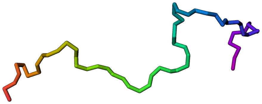
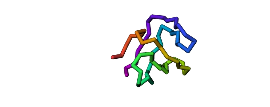
The structure pictures are the ones people like, but the contact map is the one that carries the information. Each cell is a pair of residues that touch in the folded protein. The two long bands running off the diagonal are the beta sheet that gives an SH3 domain its shape, and they are the thing that has to come back.
Watch it come apart and go back
Everything above is a number or a still. This is the thing itself: one trajectory, start to finish, the same experiment every one of the 500 runs went through. It begins at the crystal structure, is held at 1000 K until it falls apart, is dropped to 310 K, and finds its way back.
One trajectory is an anecdote
Now the part that costs money. We ran 500 of these, identical in every respect except the seed on the thermostat. Same protein, same force field, same starting structure, same temperature. If folding were a stopwatch measurement they would all land in the same place.
All 498 of them folded, and that was the last thing they agreed on. The slowest took 52 times longer than the quickest, and nothing whatsoever separated those two runs except the stream of random numbers driving the thermostat.
Run it once and you learn one number drawn from that spread, with no way to tell which one you drew.
That is the case for the ensemble being the unit of work rather than the simulation. A single trajectory cannot tell you, from the inside, whether it was the two nanosecond case or the 99 nanosecond one. Sixteen begin to show the shape. The toolkit’s own default is five hundred, and after looking at that chart the number stops looking cautious.
How fast does it fold?
Everything above counts trajectories. The thing a quench study is actually for is a rate, and the toolkit says how to get one: fit the survival curve and read the constant off it. This section is where we did that, got an exciting answer, and then found out the answer was an artefact of our own measuring stick. It is left in because the mistake is more useful than the result would have been.
Fitted by maximum likelihood, a two-population model beat a single exponential: about 95 per cent of chains folding with a time constant near 11 ns and a slow minority taking several times longer, at a likelihood ratio of 16.0 on two degrees of freedom. A slow minority is what a kinetic trap looks like from outside. It is a genuinely interesting result and we believed it.
Before trusting a fitted model, check what it predicts where you already know the answer. The folding criterion is Q ≥ 0.75 held for 750 ps, and the recorded time is the end of that hold, so no trajectory can possibly report folding earlier than the hold itself. In 500 runs the earliest fold is 1.91 ns and nothing at all lies below it. That floor is built into the definition of the measurement.
An exponential puts its mode at zero, so it must predict a pile of near-instant folds. The single exponential expects 68 of them below that floor and the two-population fit expects 75. Zero occurred. Both models are refuted by a one-line check against their own data.
And that is where the second population came from. A mixture handed a distribution with a hole at the left-hand end will spend a component filling the hole. The fast component was not a fast population of molecules; it was the model compensating for a detection delay we built ourselves. Shift the same single exponential to start at the floor and it beats the two-population model by 146 AIC with one parameter fewer: a time constant of 11.0 ns after a 1.90 ns delay.
So the honest statement is narrower than the one we nearly published. We do not have evidence for two populations. We have a folding time of roughly 11 ns once the detection delay is removed, a measurement floor that any exponential fit has to account for, and a worked demonstration that a model comparison can prefer a wrong model over a more wrong one while both are refuted.
Two caveats on the replacement, because it would be absurd to make the same error twice in the same section. The shift is estimated at the smallest observed value, which is a boundary estimate and not a well-behaved parameter, so the 146 point gap flatters it. And a floor is not the only thing that produces this shape: a chain that must pass through intermediate states before it can satisfy the criterion also produces a rising hazard. Distinguishing those needs the survival curve rebuilt from the moment Q first crosses the threshold rather than the end of the hold, which is data we have and have not yet reprocessed.
It is the folding behaviour of this coarse-grained model, at this force field scaling, under this protocol, measured through this criterion. It is not an experimental folding rate for the SH3 domain and is not comparable to one. A third shape, a stretched exponential, is reported for proteins of this class by the toolkit’s own authors (Jiang et al., Science Advances 2025) and we have not fitted it.
Can you tell in advance which chains will be slow?
There is no separate slow population, as above. There is still a tail: 20 of the 498 trajectories took longer than 41 ns. If something about the state a chain is in when the quench starts predicted which ones those would be, the spread would be set at that moment rather than during folding, and running many trajectories would be the wrong remedy: you could measure the starting state instead and save the compute. So we looked. Comparing the slowest 20 trajectories against the other 478, the radius of gyration of the unfolded chain gives p = 0.54, the residual native contacts p = 0.15, and the minimised energy p = 0.59, against a corrected threshold of 0.017. The correlation between how long a chain takes to fold and how expanded it was at the quench is r = +0.055, which is nothing.
A null is only as strong as the power behind it, so here is the power. With 20 slow trajectories against 478, at the corrected threshold and eighty per cent confidence, the smallest difference this comparison could reliably have found is about 0.74 standard deviations. Anything smaller than that would have been missed. So the claim is not that no predictor exists, it is that none of the three we can measure differs by as much as 0.7 standard deviations between the groups, and a weaker predictor would need far more slow trajectories to see, which means a much larger ensemble.
Nothing we can measure at the start of the quench says which chains get stuck, at any effect size this run could resolve. The trap looks like something the chain does on the way, not a property of where it began. That is the strongest form of the argument this whole piece is making: you cannot inspect your way out of needing the ensemble.
The stage that looked like waste
Running the toolkit’s protocol unaltered is a reproduction. This part is not: it is a question the authors did not ask, and the answer caught us out.
Every trajectory begins by heating the chain to 1000 K to pull it apart, and the toolkit budgets 60 ns for it. On our own traces the fraction of native contacts reaches zero at a median of 0.04 ns and the radius of gyration reaches ninety per cent of its plateau by 0.20 ns. The chain finishes coming apart almost immediately and then keeps going for another fifty nine nanoseconds, which is 82 per cent of every trajectory we ran. It looks like the easiest saving in the file.
Looking unfolded is not the same as being decorrelated, though. The stage also has to forget the crystal structure it started from, and a chain can look random long before it is. So we ran it: 500 more trajectories, identical except for a 6 ns unfolding stage.
| Unfolding stage | Folded | Median | Mean | Spread (sd) | Steps each |
|---|---|---|---|---|---|
| 60 nsthe toolkit’s default | 498/500 | 8.05 ns | 12.51 ns | 13.31 ns | 4,857,650 |
| 6 nsthe saving that was not there | 495/500 | 7.98 ns | 13.16 ns | 14.26 ns | 1,335,162 |
Look at the first four columns and the two protocols agree. Both fold essentially everything. The means differ by 0.74 standard errors, which is nothing. A two sample Kolmogorov–Smirnov test gives p = 0.835, which does not reject at five per cent. On that evidence the 60 ns stage is 3.6 times of waste.
Then we looked at the last column.
At a hundred trajectories per arm, the last column was where this section turned. The short protocol showed 1.33 times the spread of the long one, and a variance ratio test gave F = 1.77, p = 0.0050. We wrote it up. The 60 ns stage was not waste after all, it was doing something invisible, and we had nearly published the opposite.
Then we ran the other 400 trajectories.
At 500 against 500 the spread ratio is 1.07 and the variance ratio test gives p = 0.128. No effect. We first wrote that up as a sample size lesson: too few trajectories, a fluke, more data dissolved it. That was also wrong, and it is the more useful mistake.
Go back to the original hundred per arm and run tests that do not assume a bell curve. The F test said p = 0.005. Levene’s test, on the same numbers, said 0.33. Fligner–Killeen said 0.79. The F test assumes the data is normally distributed; folding times have a long tail, and ours had an excess kurtosis near twelve with normality rejected at p = 2×10⁻³⁵. The assumption was not approximately true, it was absent.
So the four hundred extra trajectories bought a lesson that one line of code would have given for nothing. The failure was not too little data. It was a test used outside the conditions it is valid in, and then believed because it gave the smallest number.
That is the third time the analysis on this page has been wrong in the same
way, so we stopped treating it as bad luck. Every comparison here now runs
through an assumption check before it is allowed to report anything: if normality
fails, the robust test is the answer and the parametric one is printed beside it
as a warning rather than a result. On the current data that check reports
normality fails,
so the headline p value above is Levene’s at
0.404 and not the F
test’s. The code is stats_guard.py, next to everything
else.
And a large p value is still not proof of no difference, so the interval matters more than the test. Bootstrapping the ratio of spreads gives 1.07 with a 95 per cent interval of 0.85 to 1.37. The 1.33 we originally claimed sits inside that interval, so this does not rule it out; what it rules out is our confidence in it. The interval is consistent with no difference and with a difference of thirty per cent in either direction, and anybody shortening a protocol on this evidence should know that.
Where that leaves the actual question: on the full ensemble we could not detect a difference between the two protocols on any test we ran, in mean, distribution or spread. That is not the same as showing they are equivalent, and this study was not designed to show it: an equivalence test needs a margin agreed in advance, and the two arms carry different backend mixes. So what follows is a candidate saving rather than a validated one. On this evidence the 60 ns unfolding stage can be cut to 6 ns for a 3.6 times saving on every trajectory, which is 74 per cent of the compute in a job of this shape, since the short arm still pays for its own 6 ns. We would still want somebody to check it against a protein that folds more slowly before changing a published protocol on our say-so, because a null result is a weaker thing than a positive one and we have now been wrong about this twice.
Did any of them come back knotted?
There is a reason to ask beyond curiosity. The active literature around this toolkit is largely about non-covalent lasso entanglements: a chain threading through a loop that one of its own contacts has closed. Coarse grained simulation predicted them as long-lived kinetic traps, all-atom work has since found the same states, and a 2026 paper reports that proteins carrying them misfold several times more often. If a protein has a slow population, an entangled minority is the first place to look for it.
We had just claimed a slow population and then retracted it. So this is the independent check: run the entanglement analysis on every refolded structure and see whether anything is threaded.
We did not write that analysis. The toolkit ships
calc_entanglement_number.pl, and we ran it unmodified
on our structures after first running it on its own shipped example and
reproducing the reference output byte for byte. That removes any question of our
having reimplemented the metric wrongly, which given this page’s record on
statistics felt like the right call.
One structure in 500. Replica 428 came back with 6 contacts threaded that are not threaded in the crystal structure, and every other chain returned clean.
The obvious story would be that the entangled chain is a trapped chain, and it is not. Replica 428 folded in 5.9 ns, faster than the median of 8.0 ns and quicker than seventy per cent of the ensemble. Whatever the threading cost it, it did not cost time.
One structure is not a result and we are not going to treat it as one. What it does do is agree with the retraction two sections up. If there were a real slow sub-population in this protein driven by kinetic traps, an entanglement rate of 0.2 per cent is not where it would be hiding. Two independent lines of evidence, a model comparison and a structural analysis, now point the same way: this domain folds as one population and our two-population finding was an artefact.
That is also the expected answer for a protein this small. Entanglement is reported as a phenomenon of larger, multi-domain chains, where a long tail has somewhere to thread through; the ligase in the size comparison above carries 794 native contacts against our 137. Finding almost none here is consistent with the literature rather than in tension with it, and the interesting version of this analysis is the one run on a bigger protein, which is the second row of the budget ladder below.
Turn it over yourself
The pictures above are one camera angle chosen by us. Here is the same protein with the camera in your hands. It opens on the before and after, spinning side by side at one scale. Overlay on native is the one that settles it: the refolded chain in colour, laid over the fold it started from in grey. Drag to rotate, scroll to zoom.
What the full size job costs
Our 500 trajectories are a demonstration. The number the toolkit actually ships
with is num_traj = 500, on line 291 of the same file, and that default
is the unit of work worth costing.
That figure sizes every trajectory at the full 100 ns cap. Ours did not need it: because all 498 folded and stopped early, they averaged 4.86 million steps against the 10.67 million the cap allows, which is 54 per cent less compute than the budget. Nobody could have booked that saving in advance, because you cannot know the distribution of folding times until you have measured it, and measuring it was the point. So the job is sized for the cap and billed for the mean: 395 core-hours procured, 180 actually consumed at the rate our ensemble folded. Hardware you own is sized for the cap and idle for the difference.
This page quotes 395, 180 and 155 core-hours for what is nominally the same job, so here is the reconciliation rather than leaving a reader to find it.
- 395 is what you procure: 500 trajectories each allowed the full 100 ns cap, at 3,750 steps per second per core.
- 180 is the same arithmetic on the steps the ensemble actually took, which averaged 4.86 million rather than the 10.67 million the cap allows. It is a projection, not a measurement.
- 155 is what the run consumed, summed from the wall clock of every trajectory. It is 16 per cent below the projection because 3,750 steps per second is the processor-only benchmark, and 163 of the 500 trajectories ran on the graphics backend instead. The whole machine measures 77,117 steps per second against 67,504 for the processors alone, which is 14 per cent and accounts for most of the gap.
Everything priced on this page uses the processor-only figure, so the quotes are conservative by about that margin. We would rather be wrong in that direction, and a reader who wants the other number now has both.
That is one protein, one condition, one question. The published studies this toolkit supports do that across many proteins and many conditions, and the co-translational work runs the nascent chain on a truncated ribosome, which is 4,577 beads next to the 306 of the protein itself. A system 83 times the size of the one we ran.
The useful property is that none of those 500 trajectories talks to any other one. They are independent processes with no communication, which is the easiest kind of parallelism there is. So wall clock time is not a physics constraint. It is a purchasing decision.
| Cores | Steps per second | Simulated time per second of compute | The 500 trajectory job | To reach one second of simulated time, summed over all 500 | |
|---|---|---|---|---|---|
| 1 | 3,750 | 56 ps | 16.5 days | 563 years | a single core |
| 26 | 77,117 | 1.2 ns | 19.2 hours | 27 years | this laptop, measured |
| 100 | 375,022 | 5.6 ns | 4.0 hours | 6 years | |
| 500 | 1,875,111 | 28.1 ns | 47 minutes | 14 months | one core per trajectory, and the ceiling |
Read the fourth column first. The same job, the same answer and roughly the same electricity moves from 16.5 days to 47 minutes, and nothing about the science changed. Only the number of machines somebody was willing to rent for the afternoon did. At the top of the table a researcher waits 2.4 weeks, so they ask the cheap version of the question, or asks it about one protein instead of twelve. Three rows down they ask it before lunch and argue about the answer after. That is a different research cadence rather than merely a faster one, and the thing standing between the two is procurement rather than physics.
500 trajectories means 500 independent chains, so 500 is every core this job can use. A trajectory is 10,667,000 steps that must happen in order, and a 59 bead system has nothing worth splitting across cores. Rent 50,000 cores and the job still takes about 47 minutes, for roughly a hundred times the price. Past the ceiling, more machines only buy a bigger question: more proteins, more mutants, more conditions. They cannot buy a faster answer to this one.
The science did not get easier. Somebody just rented more machines for an afternoon.
Now read the last column
That one is humbling, and it is the better answer to the question of why this work is expensive. A second is a human unit of time. Summed across all 500 trajectories, one second of simulated time takes 14 months even at the ceiling. And that is the flattering reading, because the column adds up 500 separate chains. One trajectory reaching one second takes 563 years, and no quantity of money changes that number. Chains run in order. You can buy a great many of them at once; you cannot buy a longer one.
That gap is why molecular simulation buys its speed with approximations rather than with hardware. The coarse-grained model in this piece already throws away every atom but one per residue and all of the solvent, and it still cannot reach a second. Compute moves the fourth column. It barely touches the fifth. Knowing which column a question lives in is most of knowing whether it is worth buying machines to answer it.
Coarse-grained time is not wall clock time for a real molecule. Smoothing the energy landscape speeds the dynamics up by a factor this piece has not measured, so a nanosecond here is not a nanosecond in a test tube. The column is a fair measure of what the simulation costs and an unfair one for how long a real protein takes to do anything. It is in the table because the ratios between its rows are the honest part, and those are what compute actually changes.
Why we ran it in stages
We did not start one big job and wait for it. We cut the work into stages and put them in the order of what each one would teach us. Every stage was sized so that if we had to stop there, we would still have a finished answer rather than half of one.
That is a choice, and it is worth saying why. Compute is bought before you know what you will find. A run that only pays off at the end is a bet. A run split into stages pays you at each step, and lets you stop when the answer is good enough, or keep going when it is not.
| Stage | Size | Cost | What it made possible |
|---|---|---|---|
| Warm up | 100 runs | 34 core-h | Showed the spread is real. Enough for the pictures and a first cost estimate. |
| Control arm | 100 runs | 8 core-h | The short unfolding version. Without it there is nothing to compare, so the protocol question cannot be asked at all. |
| Full ensemble | 400 runs | 121 core-h | Enough slow runs to fit a rate, and the stage whose first reading, two populations, we later withdrew. |
| Balance the control | 400 runs | 36 core-h | Makes the protocol comparison equal on both sides instead of lopsided. |
| Melting scan | 6 runs | under 1 core-h | Finds the temperature where the model comes apart. Replica exchange cannot be set up without it. |
| Replica exchange | 15 windows | days | Tests the force field we were handed, rather than only using it. |
Read the last column downwards and it is a chain. Each stage did not just add more of the same, it opened the next question. A hundred runs can show you that folding times are spread out. They cannot tell you the shape of that spread, because the slow tail is too thin to fit anything to. Five hundred can. The melting scan is worth less than an hour and nothing after it can start without it.
So the skill being shown here is not that a simulation can be run. Anyone can start a job. It is knowing what to run first, what each result makes answerable, what it will cost before committing to it, and when to stop. The whole quench study came to 199 core-hours, and at no point between the first stage and the last was there nothing to show for it.
Halfway: what the page has shown so far
You are about halfway down. Everything above this line is the experiment itself. Everything below it is what the work costs, what it cannot do, and what we would do next with a real budget. Here is the first half in six lines.
- The code runs, and we can prove it. We took a research toolkit we had never used, got it working from a cold start, and ran its own experiment. Two of the problems we hit were not in any documentation, and both are written out above so the next person does not lose the day we lost.
- The protein folds, 498 times out of 500. The median run found its shape in 8.0 nanoseconds of simulated time. The other 2 were still going when the clock ran out, and they are counted as unfinished rather than quietly dropped.
- One run would have told us nothing. The slowest run took 52 times longer than the fastest. That is the whole argument for renting computers: the answer is the shape of the pile, and a pile needs hundreds of runs.
- It is not an artefact of our machine. We ran the ensemble across two different compute backends and compared them. They are indistinguishable, which is the check that says we measured the model rather than the laptop.
- We tested part of the recipe and found it could be cheaper. One stage eats most of the compute. We built a second ensemble, 500 runs with that stage cut to a tenth, and on every test we have the two are the same. Before we got there we published the opposite result twice and had to take it back, which is further up the page where it happened.
- The whole thing cost about $70 of rented compute. Not the point, but worth saying plainly: the expensive part of this work was never the computers.
What is left: the newest result, which is the temperature where this model comes apart and the long run it set up, then what the full job costs on rented machines, where a firm like ours actually fits, what this method genuinely cannot do, and what the same instrument would answer at a budget a hundred thousand times larger.
Where this model melts
Everything above happens at one temperature. The next experiment does not, and it cannot be set up at all without a number we did not have: the temperature at which this model’s version of this protein comes apart. This phase measured it. It is the newest result on the page and it finished on 19 October 2026.
Six temperatures, 800,000 steps each, which is 12 ns apiece. They ran at once rather than in sequence, so the scan cost 13 core-minutes and 2 minutes of clock, which at the rate used throughout this page is under a cent, and we are not going to pretend otherwise. It is the cheapest thing on this page and nothing after it could start without it.
The model half unfolds at about 362 K. That is a straight-line interpolation between 350 K, where the chain still holds 0.86 of its contacts, and 370 K, where it holds 0.27. Three things to be clear about before that number travels any further.
It is a bracket, not a measurement. The grid is 20 K wide and the transition falls inside one interval of it, so the honest precision is the interval and not the decimal. A proper melting curve is an equilibrium calculation over far longer runs, which is exactly what the replica exchange job now running is for.
It is the model’s temperature, not the protein’s. A coarse-grained model has no water, no hydrogen bonds and no chemistry, and its energy scale is set by a fitted parameter. Its melting point is a property of that parameterisation. It is not comparable to a calorimetry measurement on Fyn SH3 and we are not comparing it to one.
The scan is short. 12 ns at each temperature is enough to tell folded from unfolded and not enough to call either one converged. The 370 K point, the one inside the transition, carries a standard deviation of 0.21 across its frames, which is the chain going back and forth rather than noise in the measurement.
What the number bought is the ladder. Replica exchange needs a set of temperature windows that bracket the transition, dense where the physics changes and sparse in the wings, or the replicas never swap and the method degenerates into 15 independent simulations. Ours is 15 windows from 322 to 403 K, and the spacing is not ours: we took the offsets of the toolkit’s own ladder for its example protein and recentred them on our measured 362 K, so the shape is theirs and only the centre is ours. The run reports exchange acceptance between 0.52 and 0.87, which says the windows are close enough together to swap. Whether that means they are doing their job is a separate question, and the answer turned out to be no. The next section is why.
Acceptance is not mixing, and neither is traffic
The standard way to say a replica-exchange ladder is working is to quote its exchange acceptance. We did that above. A 306 bead run has since shown that the number cannot carry the claim.
The 4C5C production run finished all 36,004 exchanges. Its pair acceptance ran 0.193 to 0.882 with a median of 0.448, comfortably inside the band anyone would call healthy. Its weakest boundary still carried 43.0 per cent of the median crossing traffic, so there was no bottleneck anywhere on the ladder. Each replica made between 10,895 and 23,403 window moves. And it completed 0 round trips: 1 of 16 replicas ever reached both ends, against a free-walk expectation of one round trip every 926 exchanges, which the run passed 39 times over.
Three diagnostics, all healthy, and the ladder still failed. Acceptance says a proposed swap was accepted. Crossing flux, which we had to write ourselves, says a replica actually changed sides at a given boundary. Per-replica mobility says it moved at all. Every one of those looked fine. The quantity that decides whether the windows can be pooled is none of them: it is whether any single replica traverses the whole ladder, because the free-energy estimator assumes the windows are sampling one connected ensemble. That is the round-trip count, and it was zero.
So a run can accept swaps at a healthy rate, carry thousands of crossings at
every boundary, move its replicas thousands of times each, and still be
16 independent simulations wearing a trench coat. We have published exchange
acceptance on this page as evidence of convergence. It is evidence that the
windows are adjacent. It is not evidence that they mixed, and
mixdiag.py now measures the difference and prints the threshold
alongside the count, so "no round trips yet" cannot be mistaken for "no round
trips and there should have been".
What this cost and what it bought. About 48 wall hours and 2 GB of trajectory, for no folding free energy. The card for that protein had predicted this before the run, on the grounds that a 213 bead protein had already made zero round trips and that mixing degrades with size. The prediction was right, which is the uncomfortable part: we ran it anyway and the honest return is a sharper diagnostic rather than a number. The standing item on this board is a sampling method that can cross a first-order transition, and this is the third independent piece of evidence that it is the real blocker rather than a better ladder.
The obvious hardware lost again
Before starting a job measured in days we ran the same bake-off this page describes further up, on the real workload this time: fifteen windows, both backends, aggregate throughput. The processor platform returned 45,000 steps per second. The graphics platform returned 20,454. That is 2.2 times in favour of the one that sounds slower, on a machine with a 40 core integrated GPU.
This is the second time on this page that the obvious accelerator has been the wrong choice for this workload, and the reason is the same both times: these systems are 59 beads, the kernels are tiny, and the cost is per-step overhead rather than arithmetic. Two minutes of measurement before a run of about 28 hours is the cheapest insurance in this business, and it is the kind of thing that never appears in a paper.
Replica exchange on this protein started at 07:14 UTC on 19 October 2026, 15 windows on the Reference platform. It finished at 11:20 UTC on 20 October 2026, having completed all 100,002 of 100,002 exchanges, turning over 3,664 exchanges an hour. Its melting point is the dashed curve in the melting section above, and it is the only result on this page that comes from it.
The analysis that will read it is already written, and was tested against
the first few hundred cycles while the run was still going:
rex_analyse.py, next to everything else. It takes the fraction
of native contacts at each of the 15 temperatures and the heat
capacity from the energy fluctuations, and reports the melting point two
independent ways. Fixing the analysis before the data exists is the cheapest
protection against tuning it afterwards until it agrees with us, and on a
page that has already had to retract three statistical claims it seemed worth
doing in the open. When it finishes, what it settles is whether the
force field scaling we inherited, nscal 1.4962, reproduces the
folding stability it was originally fitted to. That is the closed loop: the
parameter was set by a replica exchange calculation, and this is a replica
exchange calculation checking it.
What we are running next
This piece is one stage of a longer run, and the rest of it is on the same laptop. Two of the four below have now finished and are written up above, with the date they landed. The other two are running or queued, and nothing from them is claimed anywhere on this page until they are done. We list the whole queue anyway: a result you can see coming is easier to trust than one that turns up later with no warning.
| Next | Status | What it would settle |
|---|---|---|
| Balance the short arm | done | Brought the 6 ns comparison to the same size as the 60 ns one, 500 against 500, so the protocol finding stands on equal groups. The table in that section is the balanced one. |
| Find the melting point | done | Where this model comes apart. Measured at about 362 K and written up above. |
| Replica exchange, this protein | finished | The one that matters. Started 07:14 UTC on 19 October 2026, ran about 28 hours. |
| Replica exchange, their example | queued, several days | The toolkit's own worked example on its own protein, run unchanged, as a straight reproduction. |
The rented run, and why it is the one still missing
Every cloud figure on this page is arithmetic: our measured throughput multiplied by a published price list. We have never run this code on a rented machine. Until we do, those numbers are an estimate with a decimal point on it, and this box stays here saying so. When it is done, this box is replaced by the measurement and the date.
The remaining work costs about $337 of rented compute. That is the whole rest of the programme: the melting scan and both replica exchange runs. It is a rounding error against anybody’s research budget, and it buys four things we cannot get any other way.
| What the rented run settles | Why it cannot be answered from here |
|---|---|
| Whether a rented core is our core | A cloud vCPU is usually one half of a physical core sharing a cache. Our per-core rate was measured on an Apple laptop. The ratio between them is the single biggest unknown in every price on this page, and one run settles it. |
| What interruption actually costs | Interruptible instances are two thirds cheaper and can be taken away mid-run. Our launcher skips completed trajectories, so in theory losing one costs one trajectory. Nobody has ever taken an instance away from us to check. |
| Whether the wall clock collapses the way it should | The claim is that 500 independent runs finish in the time of one if you rent 500 cores. That is the central promise of the piece and it is currently a deduction, not an observation. |
| What the bill actually says | Storage, data transfer out, and the hours a machine sits idle while you set it up do not appear in a per-core price list. They appear on an invoice. |
That is the honest reason to rent a small run. Not because the science needs it, but because this page makes a cost claim and has not tested it. A measured invoice would turn the whole costing section from a careful estimate into a receipt, and a receipt is worth more to a reader deciding whether to trust us than any amount of arithmetic.
If this were somebody’s project, the wave after that
Assume the rented trial works and the numbers hold. The next step is not more of the same, it is the thing the same money buys once the unit cost is known.
| Wave | What changes | Order of cost |
|---|---|---|
| 1. The trialwhere we are | Finish this programme on rented cores and compare the invoice to the estimate. | $337 |
| 2. A second protein, end to end | Take the 213 bead enzyme through the same treatment: kinetics, protocol test, stability. Does the detection floor that produced our withdrawn two population reading behave the same way on a protein that folds more slowly, where the floor is a smaller fraction of the folding time? | tens of dollars |
| 3. A variant series | One protein, many sequence changes, the same protocol on each. This is where rented compute stops being a convenience: a hundred variants is a hundred independent ensembles and the wall clock does not have to grow at all. | hundreds |
| 4. A real question somebody is stuck on | By this point the method is calibrated, the costs are measured and the failure modes are known. That is the point at which pointing it at an unanswered question is defensible rather than hopeful. | scoped from the pilot |
Each wave is sized so the one before it has already paid for itself in information. That is the same discipline as the stages above, applied to a budget instead of a night.
The third row is the one that matters, and it needs a word of explanation. Everything on this page rests on a setting we were handed. It is called nscal, it is 1.4962 for this protein, and it comes inside the example. We did not work it out. The toolkit says where it came from: somebody ran replica exchange until the model matched a stability measured in a laboratory.
So there is a loop to close. We run the same thing ourselves and see whether we get that stability back. If we do, the chain holds from their published setting all the way to our folding times, and the number we borrowed stops being one we took on trust. If we do not, that is a more interesting result and a harder one to write up. Either way it is the difference between using somebody’s force field and testing it.
What the whole thing costs
Everything below is in core-hours. One core-hour is one hour of one processor core. The spent column is measured from the runs we have finished. The planned column uses the same measured rate and the same size scaling as the table above, so both halves are counted the same way.
| Core-hours | Rented, interruptible | Rented, on demand | |
|---|---|---|---|
| Spent so farthe 1,018-run ensemble plus every replica exchange run on the board | 3,817 | $69.58 | $170.34 |
| Still plannedthe queued rows on the board, mostly rented | 18,467 | $336.62 | $824.10 |
| Whole programme | 22,284 | $406.20 | $994.44 |
That is the number worth sitting with. This is a whole piece of research: standing up someone else’s code, measuring a folding rate, testing their protocol, and checking their force field. All of it comes to about $406 of rented compute, of which $70 is already spent.
In time rather than money it is 22,284 core-hours. On this laptop that is about 58 days running flat out. On rented machines it is a working day, if you are willing to run 2786 cores at once. Which one you buy is a scheduling choice, not a science one. That is the whole point of this piece.
And what it cost us, on our own machine
We did not rent anything. All of it ran on the laptop in the table near the top, so the real bill was electricity. That figure used to be the one number on this page we could not measure at all. The chip is now measured. The wall is still assumed, and the gap between those two sentences is the whole of what follows.
An earlier version of this page said the watts could not be measured and
gave three dead ends. Two of them are still dead. The power adapter reports
4,990 mA at 28 V no matter what the machine is doing: that is the
negotiated 140 W ceiling, not draw, and it does not move when the load
does. The battery reports zero current, because it is full and the machine is
on mains, so there is nothing flowing to measure. The third dead end was
powermetrics, which needs administrator rights. It has now been
run with them, twice.
With 89 per cent of the machine busy it reported 47.3 watts of combined processor, graphics and neural engine power: three ten second samples of 48.1, 47.3 and 46.4 W, a spread of under four per cent. An earlier sample, with 44 per cent of the machine busy, gave 33.2 W. Eight more busy cores therefore cost 14 W between them, about 1.7 W each, which is roughly what an efficiency core costs and nothing like what the headline figure per core would suggest. It is why this machine never approaches its adapter rating on work like this. The old version of this page offered a range topping out at 120 W. That top end was never reachable and is now gone.
What powermetrics does not cover is memory, storage, the
display and the adapter’s own conversion loss, so it is not a wall
figure. The band below is the measured 47 W plus an
assumed 10 to 30 W for all of that:
60 to 80 watts at the wall, with electricity at
$0.15 per kWh. The hours are measured, the chip is
measured, the uplift is a guess. Substitute your own and the arithmetic still
works, which is the only reason a range is worth printing at all. A plug-in
meter would settle the last of it in a minute and we do not have one.
| Hours of a loaded machine | Energy | Electricity | |
|---|---|---|---|
| This articleeverything run so far | 11 | 0.7 to 0.9 kWh | $0.10 to $0.14 |
| Whole programmeincluding the replica exchange | 1,238 | 74.3 to 99.0 kWh | $11.14 to $14.86 |
The electricity behind every number on this page is somewhere between 10 and 14 cents. The whole research programme, including the runs still planned, comes to $11.14 to $14.86. Rented instead, the same work is $406.
That is not a trick and it is not an argument for buying laptops. It leaves out the hardware, which costs far more per hour than the power does, and we are not quoting a figure for that because we would be inventing the purchase price and the lifetime. What it does show is the shape of this kind of work. The compute is close to free at this scale. The money goes on the time it takes to find out that the obvious backend was 2.6 times too slow, that one run in five hundred dies quietly, and that the first statistical test we reached for was the wrong one. Those took days. The electricity cost less than a bus fare.
It also buys the other half of a description. Right now we have this protein’s kinetics: how fast it folds and in how many populations. Replica exchange gives thermodynamics, the stability and the melting temperature, from the same model at the same parameter. Kinetics and thermodynamics for one molecule, internally consistent and honestly scoped, is a far more useful thing than either alone.
Where we fit
We are not a cloud provider and we do not sell compute. The work we do is the part on either side of it: getting a research code to run correctly somewhere it has not run before, turning a protocol into a job that can be launched a few hundred times without supervision, checking that the results are the results and not an artefact of the setup, and making the output legible to the people paying for it. The pictures above were part of that last step, and they took about as long to get right as the simulation did.
The compute itself is a commodity and we treat it as one. We provision on the major public clouds at their published rates, in your account or in ours with the invoice passed through. There is no markup buried in a rate, and no reseller agreement that would make one vendor the answer to every question. Which one you land on should be decided by what your job actually needs, and that is knowable before anybody signs anything.
Here is what it comes to. At the rates published on 18 October 2026, the 500 trajectory study costed out above is about $7 of rented capacity on interruptible instances, or roughly $18 at the on-demand price. The 500 trajectory pilot behind every picture on this page consumed 155 measured core-hours, which at that rate is an estimated $2.82 of rented capacity. The core-hours are measured and the dollars are not: they are the measured work multiplied by a published rate, the same distinction this page draws between a measured chip wattage and an assumed wall figure. No rental invoice exists. Interruptible is the right instrument here and the discount is around two thirds, because the trajectories are independent and our launcher already skips completed work, so losing an instance costs one trajectory rather than the run.
What a protein we have not run costs
The question a reader with their own protein will have is what theirs costs. The honest answer has two halves, and only one of them is arithmetic.
The arithmetic half is size, and it is measured rather than extrapolated. A coarse-grained force evaluation grows faster than the chain does, so a protein five times longer is more than five times dearer, not less: ours is 5.2 times longer and 7.6 times dearer. These are the three systems we benchmarked on the same day on the same machine, carried through to a 500 trajectory job at the same cap:
| System | Beads | Per step | Core-hours | Spot | 16 trajectory pilot |
|---|---|---|---|---|---|
| SH3 domain1SHF | 59 | 1.0× | 395 | $7 | $0.23 |
| Acetyltransferase3CLA | 213 | 4.6× | 1,837 | $33 | $1.07 |
| DDLB ligase4C5C | 306 | 7.6× | 2,997 | $55 | $1.75 |
| Protein | What it does | Why it is here |
|---|---|---|
| 1SHFFyn SH3 domain human · EC 2.7.1.112 | Part of Fyn, an enzyme that relays signals inside human cells. This piece of it is the grip: the bit that holds onto other proteins so the right ones meet. | The one we folded 500 times. Small, fast, reversible, and measured in laboratories for decades. |
| 3CLAChloramphenicol acetyltransferase E. coli · EC 2.3.1.28 | The enzyme that makes bacteria resistant to the antibiotic chloramphenicol, by chemically disabling the drug. | The toolkit’s own replica exchange example, and our second benchmark at 213 beads. |
| 4C5CD-alanine–D-alanine ligase E. coli · EC 6.3.2.4 | Builds a link used in the bacterial cell wall. Vancomycin works by grabbing the piece this enzyme makes, which is why the enzyme matters to resistance. | The toolkit’s flagship protein, our largest benchmark at 306 beads, and the one we scoped and declined. |
Names, enzyme classifications and organisms above were read from the RCSB PDB entry for each code rather than from the filenames in the repository.
The half that is not arithmetic is how long each trajectory has to run, and it dominates. Our SH3 domain folds in a median 8.0 ns against a 100 ns cap. A larger multi-domain protein may need ten times that window, which multiplies every figure in the table by ten, or it may not refold from a heat-denatured state at all, which for some proteins is the published result rather than a failed run. Nobody can price that off a sequence.
That is why the first thing we do is a 16 trajectory pilot. It measures the cap instead of assuming it, and at the prices above it costs single-digit dollars of compute. A quote that follows a pilot is arithmetic. A quote that precedes one is a guess with a decimal point on it.
We scoped the toolkit’s own larger protein, the D-Ala-D-Ala ligase (4C5C) in the repository’s header image, as a candidate for exactly this treatment, and did not run it. The quenching example ships a force field fitted for the SH3 domain; every 4C5C file in the repository carries the generic untuned default instead, with the fitted per-domain values living only in a log from a separate optimisation. It is three domains, one of them discontinuous. Rebuilding the model needs a secondary-structure tool we do not have installed. And the toolkit never quenches it: it folds that protein on the ribosome instead, because proteins of that class are known to get stuck. Scoping that took an afternoon and the answer was that it is a project rather than a run. Finding that out before quoting is the service.
The hours you are billed for are not the hours you use
One more gap between a core-hour figure and an invoice, measured on our own run. The 500 trajectory job took 12.2 hours of wall clock on 18 workers, which is 219 machine-hours offered. The actual work was 155 core-hours. The machine was therefore busy 71 per cent of the time it was switched on for this job.
The missing 29 per cent is the tail. Trajectories exit when they fold, so near the end of an ensemble only the slowest are still running and most of the machine stands idle waiting for them. Every figure in this piece is quoted in core-hours of real work, so none of them is inflated by that. But it matters for how you buy: rent a fixed machine by the hour and you pay for the idle cores, while a queue that hands out one trajectory at a time and bills per task does not charge you for them. On this job the difference is 64 core-hours, about 29 per cent, and it is the kind of thing that only shows up once you have run the whole ensemble rather than one trajectory.
They are arithmetic: our measured throughput against a public price list. The basis is stated so it can be checked: a 192 vCPU compute-optimised instance in a US east region, interruptible at $3.4998 an hour and $8.568 on demand, both read on 18 October 2026, divided by 192 to give the per-vCPU-hour figure every price here uses. We name the shape rather than the vendor because the capacity is a commodity and two providers quote within a few per cent of this. They are not a quote. We have not yet run this code on a rented machine, and a cloud vCPU is a hyperthread rather than a core, so the honest reading is a band of about $7 to $21 rather than a number. The conclusion survives the whole band, which is the only reason it is worth stating: the compute is not the expensive part of this work, and it is not close. The expensive part is the afternoon spent finding out that the obvious backend was 2.6 times too slow.
What rerunning it added
Running somebody else’s experiment again is only worth doing if it leaves something behind. Here is what this one did, stated plainly, so it can be judged rather than taken on trust.
It still runs, and we know what broke. The code was written
for OpenMM 7.4.1, CUDA 9.0 and Python 3.7 on a Linux cluster. We ran it on
OpenMM 8.6.1 and Python 3.14 on a laptop with no CUDA at all. One line needed
changing, because minimizeEnergy changed what unit it expects
between those versions. That is a useful thing for the next person to know, and
it has a shelf life: it will be true until the next release breaks something
else.
The obvious backend was the slow one. Running many small systems at once, the single-threaded Reference platform beat the multithreaded CPU platform by 2.6 to 1, and the ranking flips when you run one large system instead. Nothing in the repository says this, and the benchmark most people run, one job on a quiet machine, cannot show it. It is worth a factor of two and a half on the bill, which makes it the most immediately useful thing here.
A stage of the protocol can probably be shortened. The unfolding step is configured for 60 ns. Cut it to 6 ns and we cannot detect a difference in the folding times, in their average, their distribution or their scatter. We twice thought otherwise, and both times the test rather than the protein was at fault. A null result is weaker than a positive one, so this is the finding we would most like somebody to check.
The folding times have a floor, and it is ours, not the protein’s. At the full 500 runs the obvious reading was two populations, a fast one and a slow one. It did not survive a check against its own data: the criterion cannot record a fold sooner than 0.75 ns and in practice recorded none before 1.90 ns, and a two-population fit spends a component filling that hole. Correcting for the floor leaves one folding time of about 11 ns. What is new here is the sample size and the estimator, and the demonstration that the estimator can invent a population.
Mixing numerical backends was safe on one arm and not on the other, and we checked rather than assumed. On the 60 ns protocol the double and single precision runs agree as distributions. On the 6 ns arm the same test fails, with one backend carrying several times the variance of the other. A single run is not reproducible against itself, so the agreement is worth stating where it holds, and the failure is worth stating where it does not. We are not generalising either one.
Three runs in five hundred died, and only one of them said so. The other two ran to the cap and wrote ordinary looking result files full of NaN, which read as two chains that simply never folded. That is an operational fact about ensembles of this size: the dangerous failure is not the one that raises an exception, it is the one that returns a well formed number. Every analysis here now rejects a trajectory whose geometry is not finite.
What none of that is: new biology, a better force field, or a replication of a published figure. We reran one stage of one example with parameters somebody else had already fitted. The contribution is in the engineering and the method, which is the part most papers leave out and the part that costs the money.
Checking it against things we did not produce
Everything above is internally consistent, which is the weakest kind of consistent. A model can agree with itself perfectly and still describe nothing. So here are three checks against numbers that existed before we started, none of which we control, in descending order of how much they are worth.
1. Against a measurement taken in 1998
The Fyn SH3 domain is not an obscure protein, which is part of why we chose it. Its folding was measured and published nearly thirty years ago: 94.3 refolding events per second in water at 20 °C, two-state, with a folding free energy of 6.0 ± 0.6 kcal/mol (Plaxco, Guijarro, Morton, Pitkeathly, Campbell and Dobson, Biochemistry 37 (1998) 2529-2537).
Turning a rate into a time needs a convention, and the convention has to match on both sides. For a two-state process the mean waiting time is 1/k, which here is 10.6 milliseconds, while the median is ln(2)/k, which is 7.35 milliseconds. The number this page quotes for the simulation is a median, so the median is the one to compare against. Our model reaches it in 8.0 nanoseconds, which puts the model about 0.91 million times faster than the protein. On a mean-against-mean basis, our fitted 12.9 ns against 1/k, it is 0.82 million, which is the same answer.
It was wrong, and wrong in our favour, which is the worst direction. The
old number divided the experiment’s mean waiting time by our
median folding time. Mixing the two conventions inflates the ratio by
1/ln(2), a factor of 1.44, with no physics in it at all. A third-party audit
caught it. The corrected figure is
0.91 million median-to-median, or
0.82 million mean-to-mean, and both are
now generated by calibrate.py rather than written down, with the
superseded value kept in calib.json as
speedup_mixed_superseded so the correction stays auditable.
What did not change: the order of magnitude. log10 moves from 6.1 to 6.0, so “about six orders of magnitude” was and remains the honest summary. That is the reason this page leads with the exponent rather than the multiplier, and it is the one part of the original claim the error did not touch.
It is not an error. A coarse-grained model is supposed to be faster: it has thrown away the solvent, so there is no water to push out of the way, and it has smoothed the energy landscape, so there are fewer traps to escape. Both of those buy speed on purpose. The number is the price of the simplification, stated for one protein under one protocol.
It is also not the same chain, and we have now checked rather than wondered. We fold the 59 residues of 1SHF, counted from the structure file itself. The construct Plaxco and colleagues put in a stopped-flow instrument was 67 residues: their abstract names it, so this was always checkable and for a day this page said it was an open question instead. It is not. Treat the comparison below as one against a related construct of the same fold, eight residues longer, rather than against the identical molecule. Chain length moves folding rates, and we cannot say how much of the factor below is construct and how much is coarse-graining.
It is also not two medians of the same kind, and this page is in a poor
position to wave that through. The experimental median is
model-derived: ln(2)/k is the median only if the kinetics are
two-state and single-exponential, which is the 1998 paper’s own
assumption. Ours is measured, and it comes from a distribution our own
data rejects as exponential, with a Weibull shape of
1.152, a rising hazard, and
17 AIC against the
exponential. So the ratio pairs the conventions correctly and still pairs an
assumption against an observation. How much does that cost? The fitted
Weibull’s own median is
10.0 ns
— that is λ·(ln 2)1/ρ with
λ = 13.705 ns and
ρ = 1.1516, for the survival function
S(t) = exp(−(t/λ)ρ)
that lifelines fits, because a different Weibull convention
returns a different median from the same two numbers —
against the 8.0 ns we measured, so the choice of
statistic moves this comparison by tens of per cent, not by orders of
magnitude. That is the reason the exponent is the claim and the multiplier is
not, and it is the asymmetry a reader who has already met the rate section
should expect us to name rather than hope they miss.
It is also not a conversion factor. The two numbers are at different temperatures, 310 K against 293 K, and the laboratory rate is reported in water while the study it comes from derives it by analysing the guanidine dependence of folding. We have read that much off the abstract and no further, so we are not going to characterise their extrapolation for them. Treat the comparison as an order of magnitude, which is about 6 of them, and not as a multiplier to apply to somebody else’s nanoseconds. Establishing a defensible conversion needs this comparison repeated across several proteins with measured rates, which is a study and not a sentence.
What it does buy, immediately: anyone reading a coarse-grained folding time anywhere now has one worked example of how far it sits from the laboratory, and this page is no longer in the position of saying the factor is unknowable while quoting nanoseconds.
2. Against a survival fit nobody here wrote
The number this page leads with is a folding time from a survival fit with
right-censored data, and our fit is a hundred lines of maximum likelihood we
wrote ourselves. That code has been wrong three times. So we ran the same
500 trajectories, with the same 2 censored at the cap,
through lifelines, an open source survival analysis library used
well outside this field and written by people with no stake in this result.
| Quantity | Ours | lifelines | Apart |
|---|---|---|---|
| Exponential folding time | 12.916 ns | 12.916 ns | 0.00% |
They agree to the third decimal, which is what we wanted and not what we expected to be able to say after the last three months. It verifies the arithmetic and the censoring, and nothing else: both fits assume the same model, so agreement cannot tell us the model is right.
But the same library will fit a shape the exponential cannot, so we asked it to. A Weibull fit has one extra parameter, a shape, which says whether the chance of folding in the next instant rises or falls as a chain keeps going. An exponential is the special case where it does neither. On our data the shape comes out at 1.152, above one, a rising hazard, and it beats the plain exponential by 17 AIC.
That matters because it is the same conclusion our own analysis reached from a completely different direction. We found that the survival curve could not be a single exponential starting at zero, because nothing can be detected before the hold time elapses, and a shifted exponential fitted far better. A rising hazard is exactly what a shifted start produces. Two model families, two implementations, one of them not ours, pointing the same way. That is a good deal more convincing than our own fit agreeing with our own fit.
3. Against the structure itself
Relative contact order is a published property of a fold: the average sequence separation of its contacts, divided by its length. It is the number that showed folding rates across small two-state proteins track topology rather than size, and anybody can recompute it from the PDB entry. For the chain we simulated, with the standard definition of all heavy atom pairs within 6 Å, it is 0.183 over 6,677 contacts in 59 residues.
We are not claiming that as a result. It is a checkable fact about the thing we chose, which lets a reader place this protein among the others in that literature rather than take our word for it being a reasonable test case.
What is still missing, and what it would take
The stability number is the one that matters and we do not have it yet. The
force field parameter we inherited, nscal 1.4962, was fitted by its
authors to reproduce exactly the measured quantity quoted above, the folding
free energy. The replica exchange run now going is what produces our version of
it. Two honest obstacles stand between that run and the comparison.
- Our ladder does not reach the experiment. The measurement is at 293 K and our coldest window is 322 K, because the ladder was centred on the transition where replica exchange needs the sampling. Reaching the experimental temperature means either adding windows below the current bottom, which is a few more days of the same job, or reweighting down to it, which is an extrapolation outside the sampled range and would need its uncertainty stated honestly rather than hidden in a number.
- The comparison has to be reweighted, not read off. The
right tool is multistate reweighting, and we will use
pymbarrather than write our own, for the reason the previous section exists.
Until both are done, the honest statement is the one in the limits below: this model is calibrated against a published parameter and against one published rate, and not against a measurement we or anybody else made of its stability.
Could we run the rest of it?
We ran one of the toolkit’s six protocols. The fair question is whether that was a choice or a limit, so we checked every stage: what each one shells out to, whether that program is on this machine, and what the stage would cost to run. The answer is 3 of 6 run as the machine stands, and 4 of 6 once you count the substitutes we built and tested, which the three sections after this one are about. None of the remainder is blocked by anything to do with the science.
| Stage | Today | What stands in the way | Compute to run it |
|---|---|---|---|
| Build the model, fit the force fieldCG_protein_parameterization, 0 lines | blocked | Needs stride to assign secondary structure before a model can be built at all, and a WHAM implementation the repository does not ship. Neither is installed, and we have now replaced both: pydssp for the first, measured against the shipped force field in the next section, and pymbar 4.0.3 for the second. | 333 core-hours per candidate value, about $6 each |
| Build the coarse-grained ribosomeCG_ribosome_parameterization, 0 lines | runs here | Nothing missing. It needs the 50S structure and patience rather than software. | model building, no simulation |
| Fold the chain as it is synthesisedContinuous_synthesis_protocol, 0 lines | runs here | Runs, except for the rendering step, which calls vmd. That is pictures, not physics. The real obstacle is the system size: 4,577 ribosome beads next to our 59. | about 1.0 core-hours per nanosecond per chain |
| Fold it after synthesis finishesPost_translational_folding, 0 lines | runs here | Runs. The one external call is qsub, a cluster scheduler, and our own launcher already replaced that. | comparable to our quench, about 155 core-hours per 500 |
| Put the atoms backBackmapping, 0 lines | blocked | Now runs. pulchra turned out to be MIT licensed, not academic, and backmap.py has a flag to use it alone and skip pd2_ca2main entirely. We built it from source and ran the stage; the result is two sections below. | no simulation, hours |
| Measure what happenedAnalysis_protocol, 0 lines | blocked | Runs. The entanglement, native contact and chirality scripts are this directory’s own Perl, run unmodified, and the results are two sections below. The kinetic model scripts import two packages retired years ago; they now resolve through a shim onto the maintained successor, in a second interpreter, which is the architecture section further down. | no simulation |
Present and working: numpy 2.5.4, scipy 1.18.1, openmm 8.6.1, parmed 4.3.1, mdtraj 1.11.2, pdbfixer 1.12.0, matplotlib 3.11.2, pandas 2.3.3, pymbar 4.0.3, lifelines 0.30.3, deeptime 0.4.5, plus Perl, which is how the entanglement script ran.
Missing and openly licensed: a WHAM implementation
(Grossfield’s is GPL, and pymbar is already here instead),
and mkdssp under BSD-2, which would substitute for
stride with an adapter for the output format.
Missing and licence-encumbered: stride and
pd2_ca2main are academic-licence tools,
and vmd is free of charge without being open source.
For a commercial practice those are a procurement question before
they are a technical one, and we have not read each licence. Two
more, MATLAB and CHARMM, appear in alternative routes we do not need: we
replaced the MATLAB curve fit with our own, cross-checked against
lifelines, and the OpenMM route to the force field needs no
CHARMM.
Missing because of our own Python:
pyemma, msmtools, topoly publish no wheel for Python
3.12.13. The Markov state model described below wants two of those,
so it needs an older interpreter in a second environment. Cheap, and worth
knowing before promising a date.
Two things follow. The first is that the stage we skipped for scientific reasons, the force field fit, is also the one with a hard external dependency, and we should not let those two facts blur: we skipped it because the parameters were already fitted and shipped, and it would also have needed a program we do not have. The second is that the expensive-looking parts are not the expensive parts. Fitting the force field ourselves is $6 of compute per candidate value. Installing three binaries and reading their licences is the longer job.
The one genuinely large number is the co-translational protocol, and it is large for an honest reason: the ribosome is 4,577 beads. Our measured throughput falls off as roughly the 1.22 power of the bead count across the three sizes we benchmarked, which extrapolates to about 206× slower per step at that size. That extrapolation runs 15 times past the largest system we actually measured, so treat it as a floor rather than an estimate. At that rate one nanosecond of one synthesising chain is about 1.0 core-hours, which is roughly $0.02. The arithmetic from there is the reader’s to do, and it is the reason that protocol is a project.
Running it without the licensed tool
The section above says the force field stage is blocked, and that the thing
blocking it is stride: the generator checks for it and exits.
STRIDE assigns secondary structure and lists hydrogen bonds, it is free for
academic use, and for a commercial practice it is a licence to read rather than
a download. So we replaced it and measured what that costs.
The substitute is pydssp, an MIT-licensed implementation of
DSSP, the other published algorithm for the same job. We wrote a small adapter
that presents its output in the format the generator expects, ran the
generator unmodified, and compared what came out against the force field the
repository ships, which was built with STRIDE. Everything below is that
comparison.
| What was compared | Result |
|---|---|
| Secondary structure elementswhat the contact map is built from | 3 of 4 identical. The fourth differs: STRIDE calls one strand 24–30, DSSP breaks it at a bulge and calls 25–28. That is the known difference between the two algorithms rather than a fault in either. |
| The native contact setthe 50 pairs Q is counted over | 40 contacts against 50, and every one of ours is also one of theirs: 0 contacts are unique to the open source route. A strictly smaller set, not a different one. |
| What that does to the answerrecomputed over all 500 trajectories | Mean Q of the refolded structures 0.9314 against 0.9385, a mean absolute difference of 0.017. The folded call changes for 1 trajectory of 500. |
| The regenerated force fieldpair by pair against the shipped one | The same 182 interaction pairs, none added, none missing. 168 of 182 well depths identical to six decimal places. The 14 that differ do so by exactly 0.75 or 1.50 kcal/mol, which is one or two hydrogen bonds: the two algorithms disagree about 14 hydrogen bonds and about nothing else. Total well depth across the whole force field differs by -0.025 per cent. |
That is the useful form of the answer. Not “an open source substitute exists”, which is cheap to say, but: the substitution reproduces the topology exactly and the energetics to 0.02 per cent, and the entire residual is 14 hydrogen bond assignments. Anybody can check that against the two files.
The generator now runs here on open source alone, so the force field stage
is reachable. We have built the model at
5 values of nscal
(1.1954, 1.4704, 1.4962, 1.7453, 2.0322), which are the trained levels the
toolkit ships plus the value this page inherited. The scan that picks between
them is a replica exchange run at each, queued behind the one now running.
What it does not do is make the substitution invisible. A force field built this way is 0.02 per cent weaker overall and differs on 14 contacts, so results from it are comparable to ours and not identical to the authors’. Anybody reproducing this should know which tool produced which number, which is why both files are published and the manifest hashes them.
One shortcut we tried and rejected, because it would have been faster and is
wrong: nscal multiplies the contact energies, so rescaling the
shipped file looks like it should give any other value for free. It does not.
Decomposing the shipped parameters that way accounts for 72 of the 115 native
contacts exactly and leaves 43 that follow a different rule inside the
generator. A force field that is right for 63 per cent of its contacts is worse
than no shortcut at all, so we ran the generator instead.
Their analysis scripts, on our data
Two of the toolkit’s six directories are analysis rather than simulation, and we had run exactly one script out of them. Most of the rest need no external program at all, so there was no good reason not to run them. Here is what came back, including one result that is a limit on this article’s own central measurement.
Their fraction of native contacts against ours
Q is the number this whole piece rests on, and ours is a Python
reimplementation of their Perl. So we ran calc_native_contact_fraction.pl
unmodified over the same 500 refolded structures and compared frame by
frame. It found 50 native contacts,
the same as ours, and the two agree on
500 of 500 structures with a
largest difference of 0.000000. Mean Q
0.9314 against 0.9314.
That is not an interesting result and it is an important one. Every folding time, every survival curve and the headline rate on this page are derived from that number, and it is now checked against the implementation the authors wrote, not just against itself.
Chirality, which we had never looked at
A one-bead-per-residue model has very little stopping a chain from folding
into the mirror image of itself: handedness is carried by a dihedral term and
not by any atom you could point at. Their calc_chirality_number.pl
measures it, we had not run it, and on our 500 refolded structures
491 are perfectly handed and
9 are not, of which 2 are wrong
throughout. Those 9 sit at a median
2.98 Å from the crystal structure
against 2.04 Å for the rest, so the measure
is picking up something real rather than noise.
Q counts contacts inside secondary structure. Root mean square deviation from the crystal structure counts everything, and it is the check Q is not. Measured over all 500 refolded structures, the median is 2.04 Å, 466 of 500 are inside 3 Å, and 492 are inside 5 Å. The model refolds this protein to its crystal structure, which is the strongest statement this article has been able to make about accuracy rather than about kinetics.
But of the 498 structures our criterion calls folded, 6 are further than 5 Å from native and 5 are further than 8 Å. That is 1.2 per cent of them, and it is a disagreement between two criteria rather than proof that one is wrong: 5 Å is a conventional cutoff we did not derive, so this says the contact criterion does not guarantee a close structural match under a second measure, not that those runs failed to fold. The correlation between Q and deviation is only -0.40. It does not move the median folding time materially, and it is a real limit that we did not know we had until we ran somebody else’s script.
Back to all atoms
The backmapping stage was listed as blocked two sections ago, and it is not
any more. PULCHRA turned out to carry the MIT licence rather
than an academic one, and backmap.py has a flag to use it for the
whole job and skip the academic-licence tool entirely. We built it from source,
read the licence, and ran the stage.
From 59 beads it rebuilt 490 atoms across 59 residues, with C, N, O, S where a bead used to be. The carbon alpha positions move by a mean of 0.14 Å and at most 0.45 Å, so the rebuild respects what it was given rather than quietly reinventing it.
It needed one line changed. backmap.py calls
minimizeEnergy with a tolerance in energy units, which OpenMM 8
rejects because it now wants energy per unit length. That is the same
incompatibility this article documents further up in the quench driver, in a
second script, found independently. The patched copy is published beside this
page as backmap_openmm8.py with the change marked, so nobody has
to guess what we altered.
How much further this one protein could go
We ran one protocol out of six directories and one protein out of the thousands it would accept. The obvious question from anybody weighing this up is what the next step costs, so here is the ladder for this protein, cheapest first, with what each one needs that we do not already have.
| What | What it would settle | What it needs | Compute |
|---|---|---|---|
| A Markov state model of the folding routefrom data already on disk | Whether the rising hazard we found is our detection floor, as we concluded, or a genuine intermediate the chain passes through. Those two produce the same survival curve and a state model tells them apart. It is the largest open question this page leaves. | Nothing new. We kept the full trace of every run: 332,500 frames of contacts and radius of gyration at 15 ps, across the 500 trajectories. The right tool is a state model rather than a histogram, because these are relaxation trajectories and not equilibrium sampling, and treating them as equilibrium is a mistake we would rather name than make. | none days of analysis |
| Back to all atomsthe toolkit’s backmapping stage | Whether the refolded structures are physically sensible at atomic resolution, rather than plausible as beads. It also produces something a structural biologist can open and criticise. | The toolkit ships 740 lines for it and it runs on structures we already have. The dependency chain is the risk, not the compute. | hours |
| Fit the force field ourselvestheir section 1, which we skipped | The big one. nscal 1.4962 is inherited. We have now measured what it buys: the model’s folding free energy is −3.91 ± 0.10 kcal/mol against a laboratory −6.0 ± 0.6, a 3.4-sigma miss. The toolkit’s own opt_nscal.pl optimises against a binary “probability of domain stability” driven to 1.000, which our 0.9988 satisfies while spanning several kcal/mol of free energy. So the parameter was never fitted to this number, and scanning it ourselves is now the obvious way to find out whether any value reproduces it. | A replica exchange run per candidate value, which is the job now running, plus a WHAM implementation the repository does not ship. The target number is public and quoted above. | 333 core-hours each about $6 per value, 43 for a seven point scan |
| A second, independent model of the same proteinanother open source toolkit | Everything on this page is one implementation of one model. A structure-based model from a different group, built by different people from the same crystal structure, should agree on the mechanism and the melting point. Where two codes disagree is where the physics is being asserted rather than computed. | A different package entirely, its own installation, and the same care getting it right that this page documents for the first one. We would expect the setup to cost more than the compute again. | comparable to one of ours days of setup |
| Fold it on the ribosometheir sections 3 to 5 | Whether a chain built gradually out of the ribosome reaches the same place as one refolded from a denatured state. That is a real open question in the field and this toolkit was written to ask it. | A coarse-grained ribosome of 4,577 beads next to our 59, a table of codon translation times, and the messenger RNA sequence. It is a project rather than a run, which is why we scoped it and stopped. | the system is 79× larger weeks |
The pattern across all five is the same one this page keeps finding: the compute is the small, predictable number, and the expensive part is the setting up, the checking, and the discovering that an assumption was wrong. The first two rows need no compute at all and would still teach us more about this protein than another five hundred trajectories.
If you have a reason to want one of them answered, that is a conversation worth having. The first row in particular is sitting on data we already paid for.
What this does not prove
We would rather state the limits than have you find them.
This is a coarse-grained model, not a prediction about a real protein. A Cα Gō-like model is built from the answer. It is given the folded structure and asked how the chain gets there, which makes it a good tool for studying folding pathways and kinetics and a bad tool for predicting a structure you do not already have. Nothing here says anything about structure prediction.
Our folding times are not the paper’s folding times. We ran 500 trajectories against a default of 500, on one laptop rather than a cluster, and we capped the refolding window at the toolkit’s 100 ns. 498 of 500 met the criterion inside it, the slowest with 1 ns to spare. Treat the spread as a demonstration that the spread exists, which is the point being made, and not as a measured folding rate.
The core-hour figure is ours, for this protein, on this machine. It rests on 3,750 steps per second per core, measured on 18 October 2026 with 18 processes running at once on an Apple M5 Max, an Apple Silicon laptop, which is the rate a full queue actually sees. The pilot’s own average of 4,449 is higher and we do not use it: trajectories that outlive their neighbours finish against less contention, so that number flatters the job. A 306 bead protein costs about seven times more per step, as the table above shows, a GPU changes the arithmetic again, and a cloud core is not this core. The figure is an order of magnitude, honestly derived, and it is not a quote.
We have tested one setting and inherited the rest. Three choices shape every number here. One of them we have now varied, and it turned out to matter more than the result it underpins.
The folded-state threshold. To turn a simulation into a free
energy you must decide which configurations count as folded. Every 1SHF free energy
on this page was computed at Q ≥ 0.75 and nowhere else. We have since
swept it across eight values on all five existing 1SHF trajectories, which needed no
new simulation, and the result is uncomfortable: the force-field strength
that reproduces the published value ranges from 1.483 to 2.200 depending on that one
choice, against the 1.882 we built and ran. The prediction test agrees
within two standard deviations at three of the eight thresholds. At the threshold we
published, the agreement first rested on an effective unfolded count of
1.06: about one effective configuration out of 101,265 pooled.
So we ran the same simulation six times longer. On 30 October 2026, at 216,014
exchanges, the count was 5.76 and the answer was
−6.039 ± 0.069 kcal/mol, against −5.979 before. More
sampling did not move it, and it still agrees at three of the eight thresholds.
There is no published threshold for this system, which is why the spread is the
result rather than a better single number. The two thresholds with the most
unfolded sampling, 110 and 610 effective configurations (589 and 3,540 in the
longer run), both still reject the prediction.
Why they reject is not established: at those thresholds the folded-state definition
may no longer correspond to the experimental one, which would make them badly chosen
rather than the model wrong. Either way, the agreement we report below is
conditional on a choice we did not vary when we reported it, and
qsweep_curve.json holds the sweep.
The other two we have not varied. The refolding cap of
100 ns decides what counts as censored: 2 of
500 trajectories hit it, and because the fit treats those as still
folding rather than discarding them, a different cap would move the tail of the
survival curve and with it the time constant. The force field scaling,
nscal 1.4962, is the parameter that sets how strongly native
contacts attract, and it came fitted in the repository rather than from us.
Everything in this ensemble is conditional on it. The replica exchange run listed
above was the first test of that number: at 1.4962 the model misses the measured
stability by 3.4 standard deviations, which is what the calibration on the cards
then set out to address. A cap sensitivity is a second ensemble we have not yet
bought.
This was our own exercise, not client work. Nobody commissioned it and no client data touched it. Everything it used is public: the toolkit, its example files and the PDB entry.
And a reproduction is not a replication. We ran one stage of one example with parameters the authors had already fitted. That stage on its own reproduces no published result, and we are not claiming the papers are right or wrong. The comparisons with published values came afterwards and are on the cards, each with its caveats; the one that could clearly have failed, CI2, did.
Work we could do with this
What this class of model is actually used for
Before the list of things we could run, the list of things this toolkit has already been used to study, in published work by the people who wrote it. These are not our results and we are not claiming them. They are the reason a model this simple is worth running at all.
| The real problem | What the work showed |
|---|---|
| Protein that passes quality control but does not work properly | Misfolded forms can stay soluble, slip past the cell’s own proofreading, and end up less functional than they should be. A batch that looks fine by the usual checks can be partly wrong. Nissley et al., Nature Communications 2022 |
| Changing the gene without changing the protein, and changing the protein anyway | Synonymous mutations, the ones textbooks call silent, can alter the structure and function an enzyme ends up with. This matters to anybody who has ever codon-optimised a sequence to raise yield. Jiang et al., Nature Chemistry 2023 |
| Why refolded protein is worse than freshly made protein | Folding as the chain is being built is not the same as folding from a denatured state in a tube, and the two do not end up in the same place equally often. That is the central question of recovering protein from inclusion bodies. Vu et al., J. Phys. Chem. B 2023 |
| Can a small molecule stop a protein misfolding in the first place? | In this model, yes, at least in principle: a drug can steer a chain away from a tangled state it would otherwise fall into. Jiang et al., PLoS Computational Biology 2024 |
| Why folding kinetics look strange when measured carefully | Chains getting tangled around themselves explains a shape of kinetic curve that has been measured for decades and not well explained. We thought we had a small echo of this and withdrew it, which is its own illustration of how easily the shape is misread. Jiang et al., Science Advances 2025 |
Every one of those is a question about how a chain gets to its shape rather than what the shape is, and that is precisely what this class of model is for. It is also why the limits further up matter: a model that is built from the answer cannot tell you the answer, but it can tell you a great deal about the route.
And what we could run
Everything below is something this piece demonstrates rather than something we are speculating about. Each one is a question we could answer for somebody else, and each has a cost we can put a number on before starting, because we have measured the thing it scales with.
| The question | What it takes | Roughly |
|---|---|---|
| How fast does my protein fold, and in how many ways?Your structure, this protocol | A 16 trajectory pilot to measure the folding window, then the full ensemble at whatever size the pilot says is needed. | pilot under $2 ensemble $7–$55 |
| Is my protocol spending compute where it matters?A protocol audit | Pick the stage you suspect, build the control arm, run both at a size that can actually resolve a difference. This piece is a worked example, including the part where our first answer was wrong. | two arms, so roughly double a single study |
| How many runs before I can believe the answer?Ensemble sizing | The uncomfortable one. We found an effect at p = 0.005 on a hundred per arm, and the honest answer turned out to be that we had used a test our data did not qualify for. Picking a test the distribution entitles you to, before picking a sample size, is cheaper than publishing and retracting. | a pilot plus arithmetic |
| Does this published result reproduce?An independent re-run | Take a paper's claim, stand the code up from a cold start, run it, and report what happened including what broke. That is this article. | days of setup, dollars of compute |
| What does my existing job actually cost?A throughput audit | Measure your code under the load it really runs at, on the system size you really have. On this job the obvious backend was 2.6 times too slow and the GPU was idle. | an afternoon |
| A hundred variants of the same moleculeA mutant scan | The same protocol over many sequences. Nothing talks to anything else, so it divides across as many cores as you care to rent. This is the shape of problem rented compute is actually for. | one study times the variant count |
The compute figures are the honest part and the small part. Setting a research code up, checking it is doing what you think, and finding out which of your assumptions is wrong is where the time goes. That is what this page is a record of.
If you have a question of this shape, or one we have not thought of, we would like to hear it. The first conversation is free and the first piece of work is a measurement rather than a commitment.
Where this goes
What the 337 dollar run will have established
When the rented phase finishes, four things stop being estimates.
- A measured price per trajectory on hardware anyone can rent, replacing a calculation that assumes a cloud core behaves like ours.
- A tested claim that the wall clock collapses when the work is spread across rented cores, which is the central promise of this page and currently a deduction.
- A force field we have checked rather than inherited: the replica exchange run asks whether nscal 1.4962 reproduces the folding stability it was originally fitted to.
- Thermodynamics to go with the kinetics, so this protein is described two independent ways by the same model at the same settings.
What that gives us as a practice is narrower and more useful than it sounds: a costed, repeatable unit of work with a known failure rate, a published record of three occasions when our own analysis was wrong, and a calibration against a system whose answer is independently known. That is the minimum anybody should want before paying for a simulation they cannot check themselves.
Who this is for
The work suits somebody who already knows what they want simulated and does not want to hire a team to run it: a lab with a protein and a question but no spare computational person; a biotech with a protein that behaves badly in production and a suspicion about why; a group with a published method they want independently reproduced before building on it. The common thread is that the science is theirs and the engineering is the bottleneck.
What the limits below describe is this model, not this firm, and the two are worth separating. A one bead per residue model cannot compute a binding affinity or represent a reaction, and no amount of staffing changes that: it is physics, not effort. If that is your question, the answer is a different method, and choosing the right method is part of the work rather than a reason to turn it away.
On the people side: organic chemistry and the ordinary run of engineering and science analysis we handle directly, and we have analysts in the network beyond that. Anything further we hire for, and we would rather say so up front than pretend a team is larger than it is. The honest shape is that the instrument on this page is narrow and deliberately so, the bench behind it is not, and the first conversation is about which of the two your problem actually needs.
Three questions this makes askable
- Does the two-population shape survive a protein that is not a small fast domain? We thought we had found one and it turned out to be our own measurement floor. The question is still open and the method to answer it properly now exists.
- How much of a folding protocol is load-bearing? We tested one stage of one protocol and found it could be cut. Most published protocols have never had any stage tested. That is a general audit, not a one-off.
- What does changing a single residue do to the distribution, not the average? Mutation studies usually report a mean. The spread is where the mechanism is, and the spread needs ensembles, which is exactly what rented compute is for.
Dreaming bigger, costed honestly
Every figure below is compute only, at the interruptible rate used throughout this page, and divides by about eight for a protein the size of the ligase. None of it includes the human time, which is the larger number and does not scale the same way.
| Budget | Buys | What it could answer |
|---|---|---|
| Good$10,000 | 549k core-hours 25× this programme | A dozen proteins taken end to end the way this one was: kinetics, protocol audit, stability. Enough to answer the first real question, which is whether what we found here is a property of SH3 domains or of the model. Two weeks of rented time, one person. |
| Better$250,000 | 13.7M core-hours 615× | A systematic mutation library: one protein, every single-residue change, full ensembles on each. Tens of thousands of ensembles, flatly impossible on owned hardware. It maps which positions change the distribution of outcomes rather than the average, which is where misfolding lives and where a mean hides it. |
| Best$1,000,000 | 55M core-hours 2,462× | A screening platform rather than a study: every protein in a proteome of interest, folded hundreds of times each, ranked by how slow and how trap-prone. The output is not a paper, it is a searchable map of which proteins are fragile and where, which a drug programme or a manufacturing operation builds on for years. |
| Beyond$10,000,000 | 549M core-hours 62,583 core-years | The map stops being a snapshot and becomes an instrument. Every protein in a proteome, every single-residue variant of each, hundreds of replicas per variant: roughly 694 million trajectories. That is enough to ask which positions across an entire organism are fragile, and to re-run the whole thing when the force field improves, which is the part nobody can afford today. |
| No ceiling$100,000,000 | 5.5B core-hours 625,830 core-years | At this scale the coarse-grained question is finished and the money should go somewhere harder. Either the same atlas at all-atom resolution, which costs roughly a thousand times more per nanosecond and would still buy millions of runs, or a standing folding observatory: every newly deposited structure folded on arrival, every result public, re-computed whenever the method changes. A permanent, versioned record of how every known protein gets to its shape. |
The honest caveat on the last two rows is that compute stops being the constraint well before the money runs out. At ten million dollars the bottleneck is the force field, which is fitted per protein and currently needs a human judgement each time. At a hundred million it is that nobody has validated a coarse-grained model against experiment across a whole proteome, so you would be building a very precise map of a model rather than of biology. Both of those are solvable, and neither is solved by buying more cores.
The point of the ladder is not the top rung. It is that the bottom rung costs less than a laptop and the arithmetic between them is linear and public, so nobody has to take the top rung on faith.
What this method cannot do, and what it would take
These are limits of the instrument and the evidence, not of the staffing. Chemistry and routine engineering and science analysis we cover directly, analysts beyond that are in the network, and specialists we hire. Saying which constraints are physics, which are evidence, and which are simply people is the distinction most capability pages blur, so it is drawn explicitly below.
| Limit | What it would take to lift |
|---|---|
| The model is built from the answer | A Gō model is given the folded structure. It cannot predict a structure, rank a mutation it has not been told about, or say anything about a protein nobody has solved. Lifting this means a different class of model, not more of this one, and structure prediction in particular is a solved-enough problem elsewhere that the sensible move is to use those tools as an input rather than to compete with them. |
| No chemistry, no water, no electrostatics | One bead per residue cannot represent a hydrogen bond, a charge, or a drug molecule. This is a property of the model and not of the people running it. Questions about binding or catalysis need all-atom simulation, which is roughly a thousand times dearer per unit of simulated time and a different engineering problem. That is a method change and a cost, not a wall: the chemistry side we cover in house, and the all-atom engineering is the part we would scope and staff rather than improvise. |
| Simulated time is not clock time | Measured, for one protein. Coarse-graining throws away the solvent and smooths the landscape, so the model folds faster than the protein does. Against the published rate for a related construct of the same fold the factor is about 0.91 million, set out in the calibration section above. That is one protein at one temperature and not a conversion factor: a defensible one needs the same comparison across several proteins with measured rates, which is a study we have costed and not run. |
| The stability has not been checked against an experiment | Partly addressed. The folding rate is now compared against the measurement published for this domain in 1998, which is the calibration section above. The folding stability is not, and it is the one the force field was fitted to. The replica exchange run produces our side of it; the measurement is at 293 K and our coldest window is 322 K, so the comparison needs either lower windows or a reweighting with its uncertainty stated. Beyond that, a measurement on our construct rather than a published one needs a wet lab partner, which is a collaboration and not a purchase. |
| Our statistics have been wrong three times | Partly addressed, and they were not one error. They were three: a variance test used where its normality assumption did not hold, a folding-time model that could not represent the shape of its own data, and two trajectories whose arithmetic went to NaN and still wrote well formed files. Those need three different guards, not one. Every comparison now runs through stats_guard.py, which checks normality before any parametric test, reports the robust result as primary when it fails, and prints the parametric one beside it as a warning. Re-run on the data that produced the retracted finding, it flags the disagreement that should have stopped it. The fitted-model check that caught the two-population error is in the pipeline too. What it does not replace is a statistician choosing the question, and all three failures began with the wrong question rather than the wrong arithmetic. That is a hire, and on work where a number carries weight it is the one we would make first. |
| No provenance trail fit for a regulated setting | First instalment built. provenance.py writes a content-addressed manifest: SHA-256 of every force field and setup file the simulation read, of all 33 of our scripts, and of every derived file the article quotes, plus an order-independent digest over each ensemble and the exact library versions. A reader can prove they are holding the same inputs rather than assuming it, and any later edit is detectable. It is tamper-evident, not signed. A filing context also needs chain of custody, notarised timestamps and change control, none of which exist here. That remains weeks of ordinary engineering. |
Continue the research
Five directions this sets up, each one chosen because current published work is actively asking the question and because the toolkit we now have running is the kind of instrument used to answer it. These are starting points for a conversation, not a prospectus.
| Direction | The open question | Why we could take it on |
|---|---|---|
| 1. Screening proteins for entanglement traps | Coarse-grained simulation predicted that chains can thread themselves into non-covalent lasso entanglements that act as long-lived kinetic traps, and all-atom work in 2025 found those same states. Nobody has screened broadly for which proteins are prone to it. | This is a quench ensemble plus the toolkit’s own entanglement analysis, run across many proteins. The per-protein cost is the one we measured, and the work divides perfectly across rented cores. |
| 2. Does entanglement predict what the cell destroys? | Work published in 2026 reports that proteins carrying native entanglements misfold around four times more often, and that this changes whether they are degraded or persist in near-native misfolded states. The structural propensity side of that is computable. | We can produce the propensity numbers at scale. The biology side needs a partner with degradation data, which is exactly the collaboration our limits section says we lack. |
| 3. Folding on the ribosome against folding in a tube | Recent work finds co-translational folding proceeds through non-native intermediates, and that building a chain gradually may let it dodge traps that catch a chain refolding from scratch. Our experiment is the tube half of exactly that comparison. | Sections 3 to 5 of this toolkit do the ribosome half and ship a worked example. We have declined to run them so far because they are a project, which is a scoping judgement rather than a capability gap. |
| 4. Ground truth for machine-learned coarse-grained models | The fast-moving area in 2025 is learned coarse-grained force fields trained against large simulation sets. Those need carefully characterised reference ensembles, with known failure rates and documented protocol sensitivity, and such sets are tedious to produce. | Producing large, fully accounted ensembles with the failure modes written down is precisely what this page demonstrates. It is unglamorous and somebody has to do it. |
| 5. An audit of published protocols | We tested one stage of one protocol and found it could likely be shortened by 3.6 times. Most published simulation protocols have never had any stage tested, because testing one costs a second ensemble nobody budgets for. | We have now done this once, including getting it wrong and catching it. The method generalises to any protocol with a stage somebody suspects. |
Directions 1, 2 and 3 are science and would need a scientific partner. Directions 4 and 5 are method and infrastructure, which is the part we can own outright. The honest division of labour is that somebody else should be asking the biological question and we should be the reason it is affordable to ask.
Conclusion
We set out to find whether a small practice can take a published research code it has never seen, run it correctly, and say honestly what that costs. The answer is yes, and the interesting part is what it took.
The science came out roughly where the authors said it would. The protein folds. 498 of 500 valid runs reached the criterion, at a median of 8.0 ns, and the spread between the fastest and slowest is a factor of 52. We reproduced a protocol rather than a result, using a force field somebody else fitted, so this is a working installation and a calibration, not a discovery.
The engineering was where the money was. Choosing the unobvious compute backend was worth 2.6 times. Running fewer jobs at once than seemed sensible made the whole ensemble finish sooner, twice. A stage of the protocol that consumes most of the compute looks safe to shorten. None of that is in the repository, none of it is visible in a one-process benchmark, and all of it is the difference between a bill you can defend and one you cannot.
The most valuable output is the list of things we got wrong. Three findings inverted under scrutiny: a protocol effect that vanished at full sample size, a two-population result that turned out to be our own detection floor, and two dead trajectories being counted as chains that would not fold. Each is still on the page where it happened. A reader deciding whether to trust this work learns far more from those than from the parts that went smoothly, and the pipeline now refuses to publish a page that disagrees with its own data because of them.
And the compute was never the expensive part. The work so far is about $70 of rented equivalent, and the ensemble at its heart 10 to 14 cents of electricity, on the same basis as the energy table above. The expense was the time spent finding out which of our assumptions were wrong. That is the honest shape of this work, and it is the reason the first thing we sell anybody is a measurement rather than a plan.
The short version
If you read one box on this page, this is the one.
- What we did. Took a free research program we had never used, got it running, and used it to fold one small protein 500 separate times on one laptop.
- What folding is. A protein starts as a floppy chain and has to settle into one particular shape to work. Watching one chain do it is at the edge of what instruments can manage, so people simulate it as well.
- What came out. 498 of 500 runs folded, at a middle time of 8.0 nanoseconds, with the slowest taking 52 times longer than the fastest.
- Why that spread is the point. Run it once and you learn nothing. The answer is the whole distribution, and getting one means running it hundreds of times, which is what rented computers are for.
- What it cost. The ensemble, about $4 of rented-equivalent compute and 10 to 14 cents of electricity. Everything so far, about $70. With the runs still planned, $406 and $11.14 to $14.86.
- What we found that was not in the paper. The obvious compute backend is about 2.6 times too slow, the machine is only 71 per cent busy under a naive queue, and one stage of the published recipe looks safe to cut by 3.6 times.
- What we got wrong. Six things so far, listed on their own page. The first three were statistical claims, all retracted on this page rather than quietly fixed, each one still sitting where it happened with the correction attached.
- What it does not prove. This is a simplified model, built from the known answer. Its folding rate is now checked against a laboratory measurement from 1998, on a related 67 residue construct of the same fold, and comes out about 0.91 million times too fast, which is what a simplified model is supposed to do. Its stability was checked afterwards: at the strength the toolkit ships it misses the measured value by 3.4 standard deviations, which is what led to the calibration on the cards. It describes how a chain gets to its shape, not what the shape is.
- What is next. About $337 more of computing, mostly rented, none of it started. The force-field check that was next on 19 October has since run and is on the cards. A small rented run would check whether our prices are honest. Then the size of the question is set by the size of the budget.
What it would take to keep this going
This page is self-funded, which is why it is one protein and about forty dollars of compute. The instrument is now standing and the cost per question is measured, so the only thing between this and considerably more interesting work is somebody with a question and a reason to answer it. Four shapes of that, from smallest to largest.
| If this is you | What we would run | Where it starts |
|---|---|---|
| You have a protein and a questiona lab, no spare computational person | Your structure through this exact protocol: a 16 trajectory pilot to find the folding window, then an ensemble sized by what the pilot says, reported the way this page reports. | a pilot, under $2 of compute |
| You have a protocol you suspect is wastefula group with a method and a compute bill | The audit this page is a worked example of: pick the stage, build the control arm, run both at a size that can actually resolve a difference, and report it even when the answer is no. | two arms, roughly double a single study |
| You want a result independently reproduceda journal, a funder, a group building on somebody else’s claim | A cold-start reproduction with every failure written down, a content-addressed manifest of every input and output, and a published account whether or not it reproduces. | days of setup, dollars of compute |
| You want the map rather than the studya drug programme, a manufacturing operation, a funder of infrastructure | Many proteins, or every variant of one, folded hundreds of times each and ranked by how slowly and how badly they fold. This is the tier that cannot be done on owned hardware at any speed, and the arithmetic for it is in the ladder above. | $10,000 and upward |
What we would want from a partner on the science side is the question and the judgement about whether the answer is biologically interesting. What we bring is the part that makes it affordable to ask: getting the code running, making it survive a few hundred unsupervised launches, checking the result is a result and not an artefact, and saying plainly what it cost and what it did not show. If that division of labour sounds right, the first conversation is free and the first piece of work is a measurement.
Have a model that runs too slowly to ask the real question?
The symptom is usually that somebody is running three cases because three is what fits in the week, while the question actually needs three hundred. That is a solvable problem and the first step is cheap: we take your code, get it running, and measure what one run costs before anybody commits to a budget.
Start with a measurementRepeat it
The driver, the figure builder, the launcher and the rendering rig are in
folding/ next to this page. The toolkit itself, its example
files and the fitted force field are in the O’Brien Lab repository. With
OpenMM, numpy and ParmEd installed, one trajectory is one command and takes about
47 minutes on a single core at the rate we measured.
If you want to check that you are holding the same inputs we were rather than
assuming it, folding/provenance.json carries a SHA-256 of every
force field and setup file the simulation read, of every script here, and of
every derived file quoted above, along with an order-independent digest over
each ensemble and the exact library versions. Regenerate it with
python provenance.py and compare. It hashes the published copy of
the driver against the copy that actually ran and reports MATCH or
DIVERGED for each, so the code beside this article is provably the
code behind the numbers in it. It is tamper-evident, not signed, and the limits
section says what that does and does not buy you.
git clone --depth 1 https://github.com/obrien-lab/cg_simtk_protein_folding
pip install openmm numpy parmed
SETUP_DIR=cg_simtk_protein_folding/example/temperature_quenching/input/setup \
  python cgsim.py --replica 1 --outdir out
Every experiment, and when it ran
This table is generated from runlog.json, which is append-only:
once an experiment is recorded it is never rewritten, so losing the working
directory cannot quietly erase a result. 12 of these finished and
1 was withdrawn. The withdrawn one is in the table on purpose. An
experiment log that lists only what worked is a sales document, and the withdrawn
entry below is the most instructive row in it.
| Experiment | Status | Started (UTC) | Ran for | Evidence |
|---|---|---|---|---|
| rex-v1-1shfReplica exchange on 1SHF, the toolkit's example exchange count | complete | 2026-10-19 07:14 | 28.1 h | rexfit.json |
| tscan-1shfTemperature scan to locate the transition before building a ladder | complete | — | — | tscan.json |
| ens500-1shfQuench ensemble, 500 independent refolding trajectories | complete | — | — | stats.json |
| bakeoff-platformsReference against OpenCL on the real replica-exchange workload | complete | 2026-10-20 11:30 | — | rex.json |
| batch-additivityAre batched copies independent? Energies of coincident copies | complete | 2026-10-19 20:58 | — | batch.json |
| alloc-whole-machineWhole-machine allocation: CPU workers against a batched GPU context | complete | 2026-10-19 21:27 | — | alloc.json |
| rexbatch-engineBatched replica exchange in one context. WITHDRAWN: a hand-written per-DOF-kT integrator passed a kinetic-temperature gate and still sampled the wrong ensemble | withdrawn | 2026-10-20 09:52 | — | integ_diag.json |
| dt-studyDoes a larger timestep hold its accuracy? All 8 arms ran and the result is UNINTERPRETABLE: leapfrog and BAOAB disagree 1.8x on Cv at the same 15 fs and both scatter 2-3x across timesteps, against an estimated 8 per cent precision. The estimate used the velocity relaxation time, but the energy correlation time diverges near the transition, so 12 ns per arm is far too short to say anything | complete | 2026-10-20 10:54 | — | dt_study.json |
| converge-exchangesHow many exchanges the melting temperature actually needs | complete | — | — | rexfit.json |
| ladder-thinningThinning the temperature ladder, gated on round-trip mixing | complete | — | — | round_trip_v2.json |
| pilot-v2-1shfPilot on a 17-window ladder reaching the experimental temperature | complete | 2026-10-20 12:25 | 0.7 h | — |
| rex-v2-1shfFlagship v2: 13-window ladder from 293 K, convergence-sized | complete | 2026-10-20 13:32 | 7.9 h | rexfit_v2.json |
| pilot-3cla3CLA pilot: does the 1SHF ladder method transfer to 213 beads? | complete | 2026-10-20 22:26 | 1.6 h | mixing.json |
Every row names the file its numbers come from, so each line is checkable rather than asserted. Read as of 2026-10-30 21:38 UTC.
Licensing, and what it permits
We reran somebody else’s software and wrote about it commercially, so
the terms matter. Read from the LICENSE file in the clone rather
than from anybody’s description of it.
| Component | Licence | What it allows |
|---|---|---|
| cg_simtk_protein_foldingthe toolkit © 2020 Yang Jiang | MIT | Use, copy, modify, merge, publish, distribute, sublicense and sell, without restriction, including commercially and without paying anyone. The single obligation is that the copyright notice and the permission notice travel with any copy or substantial portion. |
| OpenMMthe simulation engine | permissive | Free for commercial use. Distributed under permissive terms by its authors. |
| NumPy, SciPy | BSD | Commercial use permitted, attribution preserved. No obligation to release anything of your own. |
| ParmEdreads the CHARMM files | LGPL | The one that is different. Using it and importing it in commercial work is fine. Modifying ParmEd itself and then distributing the result obliges you to release those modifications. We do not modify it, so the obligation does not arise here, but anybody building a product on this stack should know which component carries it. |
What that means in practice
Commercial use of the toolkit is explicitly permitted. MIT is about as permissive as licences get: it allows selling the software itself, let alone selling work done with it. Nobody needs permission and no fee is owed. Highland Willow could run this toolkit for a paying client tomorrow without asking anybody, and so could you.
Three things it does not give you. MIT carries an explicit disclaimer of warranty and liability, in capitals, so the authors owe nothing if a result is wrong. It is a licence to the software, not to the papers, the figures, or the fitted parameters as intellectual work, which is a separate question from copyright and one we have not had reason to test. And it is not an endorsement: the authors have not reviewed this page, do not know it exists, and any error here is ours.
What we think the obligation actually is, beyond the letter. Citing the paper the authors ask to be cited, saying plainly which parts are theirs and which are ours, and publishing the corrections when we get something wrong. The licence does not require any of that. It is the difference between what you may do and what makes the next reproduction possible.
This is a reading of the licence files, not legal advice. Anybody building a commercial product on this stack should have counsel read the LGPL component in particular.
Words used on this page
Written for anyone who arrived without a biology degree, and kept short enough to be useful as a reference. Terms are in the order you meet them above rather than alphabetical.
- Protein
- A molecule a cell builds to do a job. It starts as a long chain of smaller parts and only works once that chain has folded into the right shape.
- Amino acid
- One link in the chain. Twenty kinds exist in living things, and their order decides what shape the chain ends up in.
- Residue
- What an amino acid is called once it is joined into a chain. A 59 residue protein has 59 links.
- Folding
- The process of a floppy chain arranging itself into the compact shape it needs to work. It happens by itself, usually in millionths of a second.
- Native state
- The correct folded shape. Everything on this page is measured against it.
- Denatured
- Unfolded. A chain that has been pulled apart, by heat here, and no longer has its shape.
- Misfolding
- Settling into the wrong shape, or getting stuck on the way to the right one. Behind many diseases and a persistent problem in making protein drugs.
- Molecular dynamics
- Simulating a molecule by computing the forces on every part, nudging everything forward a tiny step, and repeating. Millions of times.
- Timestep
- How far the simulation jumps each time. Fifteen femtoseconds here, which is 0.000000000000015 seconds.
- Trajectory
- One complete simulated run, from start to finish. This page is about 500 of them.
- Ensemble
- A set of trajectories treated as one result. The central argument of this page is that the ensemble, not the trajectory, is the unit of work.
- Coarse-grained model
- A deliberately simplified molecule. Here each amino acid becomes a single bead instead of roughly twenty atoms, which makes the simulation thousands of times cheaper and throws away chemical detail.
- Go model
- A coarse-grained model built from the known folded shape: contacts present in the real structure attract, everything else repels. It is built from the answer, so it studies the route rather than the destination.
- Alpha carbon
- The backbone atom of each amino acid. In this model it is the only one kept, so a bead sits where one would be.
- Force field
- The rulebook saying how strongly each part pulls on each other part. Ours was inherited from the toolkit rather than derived.
- nscal
- The one dial in this force field that sets how strongly the native contacts attract. 1.4962 for this protein, fitted by the original authors to match a laboratory measurement.
- Native contacts, Q
- The fraction of the touching pairs from the folded shape that are present right now. Q is 1 when folded and near 0 when unfolded, and it is how this page decides whether a chain has folded.
- Radius of gyration, Rg
- How spread out the chain is. A folded protein is compact and has a small Rg; an unfolded one sprawls.
- RMSD
- How far, on average, each part of one structure sits from the matching part of another. A direct measure of how close a refolded chain got to the original.
- Temperature quenching
- The experiment on this page. Heat a protein until it falls apart, drop the temperature suddenly, and watch whether it finds its shape again.
- Langevin dynamics
- A way of simulating a molecule in a liquid without simulating the liquid, by adding random kicks and drag instead. Much cheaper, and the source of the randomness that makes every run different.
- Replica exchange
- Running many copies at different temperatures and letting them swap places, which explores shapes far faster than one copy at one temperature. The queued stage of this work.
- Melting temperature
- The temperature at which a protein is equally likely to be folded or unfolded.
- Folding stability
- How strongly a protein prefers being folded, expressed as an energy. The quantity nscal was originally fitted to reproduce.
- Survival curve
- The fraction of runs that have not folded yet, plotted against time. Fitting it gives a folding rate.
- Single and double exponential
- Two shapes a survival curve can take. One exponential means every chain faces the same odds; two means the group splits into a fast population and a slow one. We fitted both and published the two-population reading, then withdrew it: neither model survives a check against its own data. The rate section above has what replaced them.
- Maximum likelihood
- Choosing the model settings that make the observed data most probable. The correct way to fit this data, and not the way we did it first.
- Censoring
- Correctly handling runs that ended before the thing you were waiting for happened. 2 of our 500 never folded inside the time limit.
- Core-hour
- One hour of one processor core. The unit every cost on this page is quoted in.
- Interruptible instance
- Rented compute sold cheaply on the condition it can be taken back at any moment. Around two thirds off, and well suited to work that can be resumed.
- Oversubscription
- Running more work than a machine has cores for. It feels like it should be faster and is reliably slower; it cost us a factor of two, twice.
- OpenMM
- The open source engine that does the actual physics. The toolkit drives it.
- PDB
- The Protein Data Bank, the public archive of experimentally determined molecular structures. 1SHF, 3CLA and 4C5C are entries in it.
Sources
- Y. Jiang, O’Brien Lab, cg_simtk_protein_folding.
Protocol parameters cited above are read from
CG_protein_parameterization/temperature_quenching.pyandexample/temperature_quenching/input/T_quench.cntrl. - Jiang, Y., Neti, S.S., Sitarik, I. et al. How synonymous mutations alter enzyme structure and function over long timescales. Nature Chemistry 15, 308–318 (2023). doi:10.1038/s41557-022-01091-z. This is the citation the authors ask users of the toolkit to give.
- Nissley, D.A., Jiang, Y., Trovato, F. et al. Universal protein misfolding intermediates can bypass the proteostasis network and remain soluble and less functional. Nature Communications 13, 3081 (2022). doi:10.1038/s41467-022-30548-5.
- Vu, Q.V., Nissley, D.A., Jiang, Y. et al. Is posttranslational folding more efficient than refolding from a denatured state: a computational study. The Journal of Physical Chemistry B 127, 4761–4774 (2023). doi:10.1021/acs.jpcb.3c01694.
- Jiang, Y., Deane, C.M., Morris, G.M., O’Brien, E.P. It is theoretically possible to avoid misfolding into non-covalent lasso entanglements using small molecule drugs. PLoS Computational Biology 20, e1011901 (2024). doi:10.1371/journal.pcbi.1011901.
- Jiang, Y., Xia, Y., Sitarik, I., Sharma, P., Song, H., Fried, S.D., O’Brien, E.P. Protein misfolding involving entanglements provides a structural explanation for the origin of stretched-exponential refolding kinetics. Science Advances 11, eads7379 (2025). doi:10.1126/sciadv.ads7379. The stretched exponential this reports is a third shape we did not fit; see the rate section.
- Noble, M.E., Musacchio, A., Saraste, M., Courtneidge, S.A., Wierenga, R.K. Crystal structure of the SH3 domain in human Fyn. EMBO Journal 12, 2617 (1993). The structure every picture on this page is built from, solved by X-ray diffraction at 1.90 Å.
- The toolkit is published under the MIT licence, which is what makes rerunning it and writing this up permissible. We have changed one line of it, noted above, and that change is ours rather than the authors’.
- Structure 1SHF, the SH3 domain of human Fyn tyrosine kinase. RCSB PDB.
- P. Eastman et al., OpenMM, the molecular simulation engine the toolkit drives. openmm.org.
- N. Rego and D. Koes, “3Dmol.js: molecular visualization with WebGL”, Bioinformatics 31, 1322–1324 (2015). 3dmol.csb.pitt.edu. The ribbon and trace renderings on this page were produced with it; the charts and contact maps were not.
Everything this work depends on
Read from the live environment by resources.py on every build, so the
versions below are the ones that produced the numbers above rather than the ones we
remember installing. Anything whose version cannot be read says so.
Software
| Tool | What it does here | Cite |
|---|---|---|
| Python3.12.13 | the whole analysis chain | python.org |
| OpenMM8.6.1 | molecular dynamics engine for every simulation | doi:10.1371/journal.pcbi.1005659 |
| NumPy2.5.4 | all array work | doi:10.1038/s41586-020-2649-2 |
| SciPy1.18.1 | logsumexp for the MBAR mixture normalisation, cKDTree for clash detection | doi:10.1038/s41592-019-0686-2 |
| pymbar4.0.3 | multistate reweighting for every pooled free energy | doi:10.1063/1.2978177 |
| ParmEd4.3.1 | CHARMM topology parsing; restores residue names the OpenMM template matcher cannot disambiguate | github.com/ParmEd/ParmEd |
| STRIDEpresent | secondary-structure assignment; required before any model can be built, and used to generate CI2's element definitions | doi:10.1002/prot.340230412 |
| PULCHRApresent, no version banner | all-atom reconstruction from the C-alpha trace in backmapping | doi:10.1002/jcc.20906 |
| Perl5.34.1 | 15 toolkit analysis scripts are Perl | perl.org |
| Docker29.5.3 | linux/amd64 emulation for ribosome_traffic, which ships compiled for Linux only | docker.com |
| Ubuntu18.04 (container base) | the newest base still packaging libgfortran3, which ribosome_traffic needs | ubuntu.com |
| Frappe / Frappe Cloudsite API | publishing this page | frappeframework.com |
Data and databases
| Source | What we took from it | Cite |
|---|---|---|
| RCSB Protein Data Bankstructures and the search API | 1SHF, 2CI2, 1COA, 1YPA, 1NYF, 1NYG, 3CLA, 4C5C | doi:10.1093/nar/28.1.235 |
| UniProtsequence cross-references | P06241 (Fyn), P01053 and Q40059 (CI2) | doi:10.1093/nar/gkac1052 |
| ProThermDBthermodynamic database | located the CI2 wild-type literature; 35 rows for 2CI2 | doi:10.1093/nar/gkaa1035 |
| NCBI PubMed E-utilitiesprimary-source verification | every published value on this page was read from its own abstract, not from a secondary compilation | ncbi.nlm.nih.gov/books/NBK25501 |
The measurements we are testing against
| Paper | Value used, and when we verified it | Cite |
|---|---|---|
| Plaxco, Guijarro, Morton, Pitkeathly, Campbell, Dobson (1998)Biochemistry 37, 2529-2537 | Fyn SH3 folding rate 94.3 /s and folding free energy -6.0 +/- 0.6 kcal/mol. Verified from the abstract 2026-10-19. | doi:10.1021/bi972075u PMID 9485402 |
| Jackson, Fersht (1991)Biochemistry 30, 10428-10435 | CI2 folding free energy 7.03 +/- 0.16 kcal/mol by guanidinium denaturation and 7.18 +/- 0.43 by thermal denaturation, at pH 6.3. Verified from the abstract 2026-10-24. | doi:10.1021/bi00107a010 PMID 1931967 |
Tools we do not have, and what we did instead
Listing these matters more than listing the ones that worked: each is a place where this work departs from the published protocol.
- pd2_ca2main: no copy for any platform; blocks verifying backmapping against its shipped reference
- WHAM: not shipped with the toolkit; replaced by pymbar's MBAR, which is a different estimator and is labelled as a substitute
- MATLAB: used by analysis_Tq.pl; replaced with NumPy/SciPy
- CHARMM: optional path in opt_nscal; the Python route does not need it
- VMD: visualisation only, not used for any result
All simulation figures on this page come from 500 temperature quenching trajectories run on 18 and 19 October 2026 on one Apple M5 Max, 18 at a time rather than all at once, taking 12.2 hours of wall clock for 155 core-hours of work. 500 of those 500 produced usable physics and the rest are accounted for above. Throughput figures are measured under the load of a full queue rather than on an idle machine, because this page found that the difference between those two is a factor of two and a half. This piece is a companion to Moore’s Law at 55, which is the argument for why renting burst compute now beats waiting for hardware to get cheaper.